
This sample Statistical Techniques and Analysis Research Paper is published for educational and informational purposes only. If you need help writing your assignment, please use our research paper writing service and buy a paper on any topic at affordable price. Also check our tips on how to write a research paper, see the lists of psychology research paper topics, and browse research paper examples.
Statistics? What does statistics have to do with psychology? Perhaps you have heard this question. It is a fairly common one and usually reflects the belief that psychologists are people who help others with emotional problems, mostly by talking with them. Why would such a person need to know about statistics? Of course, as this two-volume work shows, psychologists have many other interests and do many other things besides helping people with emotional problems. Nevertheless, even if psychologists restricted themselves to this one endeavor, statistics would be a necessary component of their field because the particular techniques that clinical and counseling psychologists use were selected after being tested and compared with other techniques in experiments that were are analyzed with statistics.
Of course, because psychologists are interested in memory, perception, development, social relations, and many other topics as well as emotional problems, they design and conduct experiments to answer all kinds of questions. For example,
- What events that occur after an experience affect the memory of the experience?
- Do people experience visual illusions to different degrees?
- In children, do the number of neural connections decrease from age 12 months to age 36 months?
- Do people work just as hard if an additional member joins their team?
To answer questions such as these, psychologists who study memory, perception, development, and social relations design experiments that produce data. To understand the data and answer the questions, statistical analyses are required. Thus, statistics courses are part of the college education of most every psychology major. In addition to being necessary for answering psychological questions, statistical analyses are used in a variety of other fields and disciplines as well. Actually, any discipline that poses comparative questions and gathers quantitative data can use statistics.
Definitions
Statistics and Parameters
Statistics has two separate meanings. A number or graph based on data from a sample is called a statistic. In addition, statistics refers to a set of mathematical techniques used to analyze data. Thus, the mean and standard deviation of a sample are statistics, and t tests and chi square tests are statistics as well.
A number or a graphic that characterizes a population is called a parameter. Parameters are usually symbolized with Greek letters such as p (mean) and a (standard deviation). Statistics are usually symbolized with Latin letters such as M or X (mean) and SD or s (standard deviation).
Populations and Samples
The goal of researchers is to know about populations, which consist of all the measurements of a specified group. Researchers define the population. A population might consist of the size of the perceived error of all people who look at a visual illusion; it might be the work scores of all people who have an additional member join their team. Unfortunately, for most questions, it is impossible or impractical to obtain all the scores in a population. Thus, direct calculation of p or a is usually not possible.
The statistical solution to this problem is to use a sample as a substitute for the population. A sample is a subset of the population. Calculations (such as M) based on sample data are used to estimate parameters (such as p). In actual practice, researchers are interested not in an absolute value of p but in the relationships among p’s from different populations. However, basing conclusions about p’s on sample data introduces a problem because there is always uncertainty about the degree of the match between samples and their populations. Fortunately, inferential statistical techniques can measure the uncertainty, which allows researchers to state both their conclusion about the populations and the uncertainty associated with the conclusion.
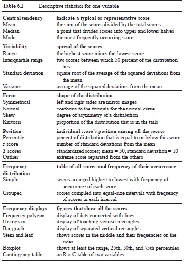
Table 6.1 Descriptive statistics for one variable
Descriptive Statistics and Inferential Statistics Techniques
Descriptive statistics are numbers or graphs that summarize or describe data from a sample. The purpose of descriptive statistics is to reveal a particular characteristic of a sample or a score with just one or two numbers or a graph. Table 6.1 is a catalog of commonly used descriptive statistics for one variable.
Researchers often gather data from two distributions to determine whether scores in one distribution are related to scores in the other distribution (correlation) or to determine the degree of difference between the two distributions (effect size index). Table 6.2 is a catalog of commonly used descriptive statistics for two variables.
Inferential statistical techniques provide quantitative measures of the uncertainty that accompanies conclusions about populations that are based on sample data. Common examples of inferential statistical techniques include chi square tests, t tests, analysis of variance (ANOVA), and non-parametric tests.
Sampling Distributions and Degrees of Freedom
A sampling distribution (also called a probability density function) shows the results of repeated random sampling from the same population. For a particular sampling distribution, each sample is the same size and the same statistic is calculated on each sample. If the statistic calculated is M, then the sampling distribution (in this case, a sampling distribution of the mean) allows you to find the probability that any particular sample mean came from the population. Sampling distributions provide the probabilities that are the basis of all inferential statistical techniques.
One attribute of every sampling distribution is its degrees of freedom, which is a mathematical characteristic of sampling distributions. Knowing the degrees of freedom (df) for a particular data set is necessary for choosing an appropriate sampling distribution. Formulas for df are based on sample size and restrictions that a model imposes on the analysis.
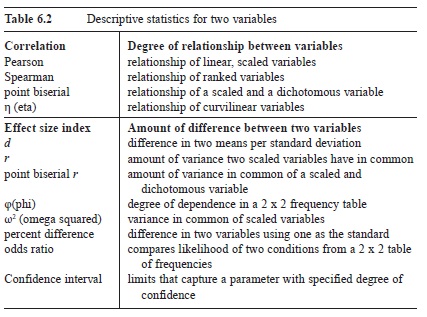 Table 6.2 Descriptive statistics for two variables
A Brief History Of Inferential Statistical Techniques
An examination of scientific reports before 1900 that include statistical analyses reveals a few familiar descriptive statistics such as the mean, median, standard deviation, and correlation coefficient but none of today’s inferential statistical techniques. In 1900, however, Karl Pearson introduced the chi square goodness-of-fit test. This test objectively assessed the degree of fit between observed frequency counts and counts expected based on a theory. Using the test, researchers could determine the probability p) of the data they observed, if the theory was correct. A small value of p meant that the fit was poor, which cast doubt on the adequacy of the theory. Although the logic of this approach was in use before 1900, the chi square test was the first inferential statistical technique whose sampling distribution was based on mathematical assumptions that researchers could reasonably be assured were fulfilled. Chi square tests today are a widely used tool among researchers in many fields. The path that Pearson used to establish chi square tests revealed the way for others whose data were statistics other than frequency counts. That is, for those who wanted to use this logic to determine the probability of sample statistics such as means, correlation coefficients, or ranks, the task was to determine the sampling distribution of those statistics.
Of those efforts that are today part of the undergraduate statistics curriculum, the second to be developed was Student’s t test. William S. Gosset was an employee of Arthur Guinness, Son & Company, where he applied his knowledge of chemistry and statistics to the brewing process. From 1906 to 1907, he spent several months in London working with Pearson. In 1908, using the pseudonym “Student,” he published sampling distributions of means calculated from small samples. The result was that experiments that had one independent variable (IV) with two levels could be analyzed with a test that gave the probability of the observed difference, if it were the case that the two samples were from the same population. To derive these sampling distributions, Student (1908) assumed certain characteristics about the population. One of these was that the population was normally distributed.
In 1925 Ronald A. Fisher published Statistical Methods for Research Workers, a handbook that included summaries of his earlier work. This example-based instruction manual showed how to analyze data from experiments with more than two levels of the IV (one-way ANOVA) and experiments with more than one IV (factorial ANOVA). In addition, it showed how to remove the effects of unwanted extraneous variables from the data (analysis of covariance). Fisher’s (1925) book was incredibly influential; 14 editions were published, and it was translated into six other languages.
Perhaps more important than Fisher’s description of a general approach to analyzing data, regardless of the kind of experiment the data came from, was his solution to the problem of extraneous variables in experiments. In a simple but ideal experiment, there is an IV with two levels and one dependent variable (DV; see Chapter 9). The researcher’s hope is to show that changes in the levels of the IV produce predictable changes in the DV. The most serious obstacle to establishing such cause-and-effect conclusions is extraneous variables, which are variables other than the IV that can affect the DV. In the worst case, an extraneous variable is confounded with the IV so that there is no way to know whether changes in the DV are due to the IV or the confounded extraneous variable. Fisher’s designs either balanced the effects of extraneous variables over the different levels of the IV such that there was no differential effect on the DV or they permitted the effects of the extraneous variables to be removed from the analysis. It is not too strong to say that Fisher’s methods revolutionized science in agronomy, biology, psychology, political science, sociology, zoology, and the other fields that rely on statistical analyses.
The logic of the approach of that Fisher and Gosset used was to tentatively assume that the samples observed came from populations that were identical (a hypothesis of no difference). A sampling distribution based on a hypothesis of no difference shows the probability of all samples from the population, including the one actually observed. If the probability of the actually observed sample is small, then support for the tentative hypothesis is weak. Following this reasoning, the researcher should reject the tentative hypothesis of no difference and conclude that the samples came from populations that were not identical.
What is the dividing point that separates small probabilities from the rest? Fisher’s (1925) answer in Statistical Methods for Research Workers was to mention a value of p = 0.05 and continue with “.. .it is convenient to take this point as a limit in judging whether a deviation is to be considered significant or not” (p. 47). However, Fisher’s own practice, according to Salsburg (2001), was to recognize three possible outcomes of an experiment: small p, large p, and intermediate p. A small p such as < 0.05 led to rejection of the hypothesis of no difference. A large p such as .20 or greater led to the conclusion that if the treatments actually made a difference, it was a small one. An intermediate case of 0.05 < p < .20 led to the conclusion that more data were needed (Salsburg, 2001). Remember that the accuracy of these probability figures is guaranteed only if certain assumptions about the populations are true.
In 1933 Jerzy Neyman and Egon Pearson (son of Karl Pearson) proposed revisions and extensions to Fisher’s approach. They noted that in addition to the hypothesis of no difference in the populations, there is an unemphasized hypothesis—there is a difference in the populations. The follow-up to this seemingly trivial point led to developments such as Type I errors, Type II errors, and power, which are explained below.
Neyman and Pearson referred to the hypothesis of no difference as the null hypothesis and the hypothesis of a difference as the alternative hypothesis. Taken together, these two are exhaustive (they cover all possibilities) and mutually exclusive (only one can be true). Noting that there are two hypotheses revealed clearly that an experiment was subject to two kinds of errors. Rejecting the null hypothesis when it was true (due to an unlucky accumulation of chance) became known as a Type I error, an error that was clearly recognized by Fisher. However, failure to reject a false null hypothesis is also an error, and Neyman and Pearson called this an error of the second type (a Type II error). Identifying and naming the Type II error pushed statistical practice toward a forced decision between two alternatives: reject the null hypothesis or fail to reject it. In addition, recognizing the Type II error, which can occur only when the null hypothesis is false, led the way to an analysis of statistical power, which is the probability of rejecting a false null hypothesis.
In 1934 Neyman introduced the confidence interval (Salsburg, 2001). Calculated from sample data and utilizing a sampling distribution, a confidence interval is a range of values with a lower limit and an upper limit that is expected to contain a population parameter. The expectation is tempered by the amount of confidence the sampling distribution provides. Researchers most commonly choose a 95 percent level of confidence, but 90 percent and 99 percent are not uncommon.
In the 1940s another group of sampling distributions were derived so that probabilities could be determined for data that consisted of ranks rather than the more common, relatively continuous measures such as distance, time, and test scores. Frank Wilcoxon (1945) and Henry B. Mann and D. Ransom Whitney (1947) published tests that are appropriate for ranks. These tests were different from previous ones in that the populations sampled are not normally distributed and no population parameters are estimated. These tests are called nonparametric tests or distribution-free tests.
Null Hypothesis Statistical Testing (NHST)
In today’s textbooks the process that developed over some 50 years is referred to as null hypothesis statistical testing (NHST) and is often treated as a rule-based method of reaching a decision about the effect of the IV on the DV. NHST begins with the two hypotheses about the populations the data are from—the null hypothesis of no difference (H0) and the alternative hypothesis that the populations are not the same. NHST also begins with a criterion that the researcher chooses for deciding between the two. This criterion is a probability, symbolized a (alpha). The sample data are analyzed with a statistical test that produces a probability figure, p, which is the probability of the data that were observed, if the null hypothesis is true.
If the value of p is equal to or less than the value of a, the null hypothesis is rejected and the alternative hypothesis is accepted. In this case, the test result is statistically significant.
If the value of p is greater than a, the null hypothesis cannot be rejected, so it is retained. This outcome, p > a, produces an inconclusive result because both hypotheses remain. Note, however, that although the logic of NHST has not led to a rejection of the null hypothesis, the researcher does have the sample data, which give hints about the populations. In the case of p > a, NHST procedures do not permit a strong statement about the relationship of the parameters in the population.
Table 6.3 summarizes the four outcomes that are possible with NHST tests. There are two ways to make a correct decision and two ways to make an error. The probability of a Type I error (a) is chosen by the researcher. The probability of a Type II error is (1, which is discussed under the topic of power.
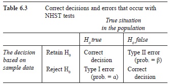 Table 6.3 Correct decisions and errors that occur with NHST tests
The developers of statistical techniques all emphasized that their procedures were to be aids to decision makers and not rules that lead to a decision. However, subsequent researchers and textbook writers began using NHST logic as an algorithm—a set of rules that lead to a conclusion that is correct with a specified degree of uncertainty. In this rigid view, if p < a, reject the null hypothesis. If p > a, retain the null hypothesis. As mentioned earlier, however, the very basis of the decision rule, sampling distributions and their p values, are themselves dependent on the mathematical assumptions that allow sampling distributions to be derived. If the assumptions don’t hold, the accuracy of the probability figure is uncertain. It is the case that every statistical test is based on some set of assumptions about the nature of the population data, and some of these sets are more restrictive than others.

Assumptions Underlying Sampling Distributions
A sampling distribution is a formula for a curve. Using a sampling distribution, researchers or statisticians determine the probability of obtaining a particular sample (or one more extreme) in a random draw from the population. To derive a sampling distribution, mathematical statisticians begin with a particular population. The characteristics of that population are assumed to be true for the population that the research sample comes from. For example, the sampling distributions that Gosset and Fisher derived for the t test and the analysis of variance assumed that the populations were normally distributed. If the populations the samples come from have this characteristic (and others that were true for the populations from which the sampling distribution was derived), then the probability figure the sampling distribution produces is accurate.
Although there are statistical tests to determine the nature of the populations the samples come from, the data available for the test are often limited to the research samples. If these data are ample, these tests work well. If ample data are not available, the tests are of questionable value. However, for some measures that are commonly used by researchers, there is more than enough data to assess the nature of the populations. For example, we know that IQ scores are normally distributed and that reaction time scores and income data are skewed.
The question of what statistical test to use for a particular set of data is not easily answered. A precise solution requires knowing the mathematical assumptions of each test and that the assumptions are tenable for the population being sampled from. Researchers, however, are usually satisfied with a less precise solution that is based on the category of the data and the design of the experiment.
Data Categorization
The recognition that some kinds of data cannot meet certain assumptions led to efforts to categorize data in such a way that the test needed was determined by the category the data fit. Two different category schemes have emerged.
Probably the most widely used scheme has three categories: scaled data, rank data, and category data.
Scaled data are quantitative measures of performance that are not dependent on the performance of other subjects. Measures of time, distance, errors, and psychological characteristics such as IQ, anxiety, and gregariousness produce scaled data. Rank data (also called ordinal data) provide a participant’s position among all the participants. Any procedure that results in simple ordering of 1, 2, 3…produces rank data. Situations in which participants order a group of items according to preference, creativity, or revulsion produce rank data. Class standing and world rank are examples of rank data. Category data (also called nominal data) consist of frequency counts. A variable and its levels are defined and the number of subjects or participants who match the definition is enumerated. A variable such as gender with frequency counts of males and females is an example, as is the number of individuals who check agree, no opinion, or disagree on a Likert scale.
Listing the categories in the order of scaled, rank, and category puts them in the order of more information to less information. Given a choice, researchers prefer to use measures with more information rather than less, but many times the circumstances of their research designs leave them no other practical choice.
The other common way to categorize data is with four scales of measurement. The first scale, nominal measurement, corresponds to category data. The second scale, ordinal measurement, has the same definition as that for rank data. The interval scale of measurement has scaled scores with two characteristics. The first characteristic is that the intervals between equal scores are equal. The second is that the score of zero is arbitrarily defined and does not mean an absence of the thing measured. Common examples of interval scales are the Celsius and Fahrenheit temperature scales. In neither case does zero mean the complete absence of heat and, of course, the two zeros don’t indicate the same amount of heat. However, a rise of 10 degrees from 20 to 30 is the same amount of heat as a rise of 10 degrees from 80 to 90 for Celsius and for Fahrenheit scales. The ratio scale consists of scaled scores as well, but zero on the ratio scale means the complete absence of the thing measured. Errors (both size and number), reaction time, and physical measures such as distance and force are all measured on a ratio scale.
Experimental Design
Besides the kind of data produced, researchers select a statistical test according to the design of their experiment. In some experiments, each of the scores is independent of the others. That is, there is no reason to believe that a score could be predicted by knowing an adjacent score. In other experiments, such a prediction is quite reasonable. Experiments in which one twin is assigned to the experimental group and the other to the control group can be expected to produce two similar scores (although one score may be expected to be larger than the other). Other designs that produce related scores are before-and-after studies and matched pair studies in which each participant assigned to the experimental group is matched to a participant in the control group who has similar characteristics.
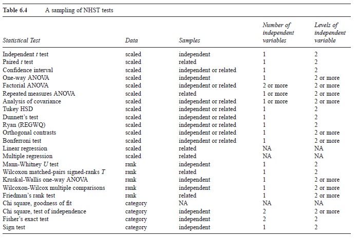 Table 6.4 A sampling of NHST tests
In addition to the independent/related issue, experimental designs differ in the number of IVs, which can be one or more. Designs also differ in the number of levels of each IV. The number of levels can be two or more.
Researchers often choose a particular NHST test by determining the kind of data, whether the scores are independent or related, and the number and levels of the IV(s). Table 6.4 is a catalog of NHST tests, many of which are covered in undergraduate statistics courses. Those tests that require scaled data have somewhat restrictive assumptions about the populations the samples are from.
Robust Tests
A robust statistical test produces accurate probabilities about the population even though the population does not have the population characteristics the sampling distribution is based on. For example, a test that assumes the population is normally distributed is robust if a sample produces a correct p value, even if the population that is sampled from is not normally distributed.
A common way to test robustness is to begin with populations of data created with characteristics unlike those the sampling distribution was derived from. A computer program randomly and repeatedly samples from the population, a technique called the Monte Carlo method. With a large number of samples at hand, the proportion of them that produces test values of, say, 0.05 or less is calculated. If that proportion is close to 0.05, the test is robust, which is to say that the test is not sensitive to violations of the assumptions about the population that the test is based on. As might be expected, when robustness is evaluated this way, the results depend on the degree of “unlikeness” of the sampled populations. A common conclusion is that for research-like populations, statistical tests are fairly robust. That is, they are relatively insensitive to violations of the assumptions they are based on. In general, NHST tests are believed to give fairly accurate probabilities, especially when sample sizes are large.
Power
The best possible result with NHST is to reject H0 when the null hypothesis is false. In Table 6.3, this fortunate outcome is in the lower right corner. As seen in Table 6.3, the other possible result is a Type II error, the probability of which is (1. Thus, when the null hypothesis is false, the probability of reaching a correct decision is 1(1. This probability, 1(1, is the power of a statistical test. In words, power is the probability of rejecting a false null hypothesis.
There are two answers to the question, “How much power should a researcher have for an NHST test?” One answer is that the amount of power should reflect the importance of showing that the null hypothesis is false, if indeed it is false. The second answer is to use a conventional rule-of-thumb value, which is 0.80.
Calculating the numerical value of the power of a particular statistical test is called a power analysis. It depends on a number of factors, only some of which are under the control of the researcher. For an NHST test that compares two groups, four of the factors that influence power are the following:
- Amount of difference between the populations. The greater the difference between two populations, the greater the chance that this difference will be detected. Although researchers do not know exactly how different populations are, they can estimate the difference using sample means.
- Sample size. The larger the sample, the greater the power of the test to detect the difference in the populations. Sample size is incorporated into the value of the statistical test used to analyze the data.
- Sample variability. The less the variability in the sample, the greater the power of the test. Sample variability, like sample size, is incorporated into the statistical test value.
- Alpha (a). The larger the value of a, the greater the power of the test. To explain, rejecting H0 is the first step if you are to reject a false null hypothesis. Thus, one way to increase power to 1.00 is to reject H0 regardless of the difference observed. As seen in Table 6.3, however, rejecting H0 when the null hypothesis is true is a Type I error. Even so, if a researcher is willing to increase the risk of a Type I error by making a larger, more tests will result in decisions to reject H0. Of course, for every one of these cases in which the populations are different, the decision will be correct.
The relations among power and these four factors are such that setting values for any four of them determines the value of the fifth. Determining one of the five values is called a power analysis. In practice, researchers use a power analysis to determine the following:
- Sample size when planning a study. Using previous data or conventional rules of thumb, the sample size required for power = .80 (or some other amount) is calculated.
- Power of a study in which H0 was retained. High power and a retained H0 lend support to the idea that any difference in the populations must be small. Low power and a retained H0 lend support to the idea that a Type I error occurred.
Other Statistical Techniques
Most undergraduate statistics courses emphasize statistical techniques that compare the means of two or more treatment groups. However, other techniques are available. Regression techniques permit the prediction of an individual’s score based on one other score (simple regression) or on several scores (multiple regression). Structural equation modeling allows researchers to test a theoretical model with data and then use the data to modify and improve the model. Other techniques are used for other purposes. The underlying basis of most statistical techniques is called the General Linear Model. The NHST techniques discussed in this research-paper are all special cases of the General Linear Model, which might be considered the capstone of 20th-century mathematical statistics.
Computer-Intensive Methods
The basis of NHST statistics is a sampling distribution. Traditionally, sampling distributions are mathematical formulas that show the distribution of samples drawn from populations with specified characteristics. Computer-intensive methods produce sampling distributions by repeatedly and randomly drawing samples from a pseudopopulation that consists of data from the experiment. A particular method called bootstrapping illustrates this approach. With bootstrapping, as each score is selected it is replaced (and can be selected again).
To illustrate, suppose a researcher is interested in the mean difference between two treatments. Data are gathered for each treatment, the means calculated, and one is subtracted from the other. If the two samples are from the same population (the null hypothesis), the expected difference between the two sample means is zero. Of course, two actual means will probably differ. To generate a sampling distribution that shows the entire range of differences, all the sample data are used to create a pseudopopulation. A computer program randomly draws many pairs of samples, calculates the two means, and does the subtraction. The result is a sampling distribution of mean differences. Finally, the difference between the two treatment means obtained in the experiment can be compared to the mean differences in the sampling distribution. If the difference obtained in the study is not likely according to the sampling distribution, reject H0 and conclude that the two treatments produce data that are significantly different. Thus, computer-intensive methods are also based on NHST logic.
Meta-Analysis
Meta-analysis is a statistical technique that addresses the problem of how to draw an overall conclusion after researchers have completed several studies on the same specific topic. It is not unusual for a series of studies to produce mixed results; some reject the null hypothesis and some retain it. Meta-analysis is a statistical technique pioneered by Glass (1976) that combines the results of several studies on the same topic into an overall effect size index. This averaged effect size index (often an averaged c/value, d) is reported with a confidence interval about it. A d value is interpreted in the same way as a d value from one study. The confidence interval about d is interpreted in the same way as a confidence interval about a mean.
The NHST Controversy
In the 1990s a controversy erupted over the legitimacy of NHST. The logic of NHST was attacked, and researchers who misinterpreted and misused NHST were criticized. One of the central complaints about the logic of NHST tests was that the best they could provide was a conclusion that could be arrived at logically without any data analysis. The case can be made that for any two empirical populations, the null hypothesis is always false if you carry enough decimal places. If this is true, the best that NHST can do is to confirm a conclusion that could have been reached on logical grounds—that the populations are different.
A second complaint about the NHST procedure is that it always starts at square one, ignoring any previous work on the variables being investigated. As a result, a sequence of experiments on the same variables, analyzed with NHST techniques, does not lead to more precise estimates of parameters, but only to more confidence about the ordinal positions of the populations.
A third problem with the logic of NHST is that it focuses on minimizing the probability of a Type I error, the error of rejecting a true null hypothesis. Of course, if two populations are different (as noted in the first complaint), Type I errors cannot occur. In addition, focusing on Type I errors leaves evaluation of Type II errors as an afterthought.
The most prevalent misunderstanding of NHST is of the p in p < 0.05. The p is the probability of the test statistic when the null hypothesis is true. It is not a probability about the null hypothesis. It is not the probability of a Type I error, the probability that the data are due to chance, or the probability of making a wrong decision. In NHST, p is a conditional probability, so p is accurate only when the condition is met, and the condition is that the null hypothesis is true.
Another complaint, alluded to earlier, is about the practice of using the 0.05 alpha level as a litmus test for a set of research data. The practice has been that if an NHST test does not permit the rejection of H0, the study is not published. This practice can deprive science of the data from well-designed, well-run experiments.
As a result of the complaints against NHST, the American Psychological Association assembled a task force to evaluate and issue a report. Their initial report (http://www.apa.org/science/bsaweb-tfsi.html) recommended that researchers provide more extensive descriptions of the data than just NHST results. They recommended increased reporting of descriptive statistics, such as means, standard deviations, sample sizes, and outliers, and a greater use of graphs, effect size indexes, and confidence intervals. In their view, NHST techniques are just one element that researchers use to arrive at a comprehensive explanation of the results of a study and should not be relied on exclusively.
The Future
As the reader has no doubt detected, the field of statistics has been a changing, dynamic field over the past one hundred years. The future appears to be more of the same. As an example, Killeen (2005) described a new statistic, prep, which has nothing to do with null hypothesis statistical testing. The statistic, prep, is the probability of replicating the results that were observed. In particular, prep is the probability of finding a difference with the same sign when the control group mean is subtracted from the experimental group mean. Thus, if the original experiment resulted in Xe = 15 and Xc = 10, then prep is the probability of Xe > Xc if the experiment were conducted again.
This new statistic, prep, is one response to the complaints about NHST logic described earlier. It has a number of advantages over the traditional p value from a NHST analysis, including the fact that because there is no null hypothesis, there are no Type I and Type II errors to worry about. It is a continuously graduated measure that does not require a dichotomous reject/not reject decision. Finally, the calculation of prep permits the incorporation of previous research results so that the value of prep reflects more than just the present experiment. The statistic prep appears to be catching on, showing up regularly in Psychological Science, a leading journal.
As the 21st century began, the prevailing statistical analysis was NHST, a product of 20th-century statisticians. As for the future, new statistics are always in the works. NHST may not remain the dominant method for analyzing data; other statistics may supplant it, or it may continue as one of the techniques that researchers use to analyze their data.
References:
- Fisher, R. A. (1925). Statistical methods for research workers. London: Oliver and Boyd.
- Glass, G. V. (1976). Primary, secondary, and meta-analysis of research. Educational Researcher, 5, 3-8.
- Killeen, P. R. (2005). An alternative to null-hypothesis significance tests. Psychological Science, 16, 345-353.
- Mann, H. B., & Whitney, D. R. (1947). On a test of whether one or two random variables is stochastically larger than the other. Annals of Mathematical Statistics, 18, 50-60.
- Neyman, J., & Pearson, E. S. (1933). On the problem of the most efficient test of statistical hypotheses. Philosophical Transactions of the Royal Society, A 231, 289-337.
- Salsburg, D. (2001). The lady tasting tea: How statistics revolutionized science in the twentieth century. New York: W. H. Freeman.
- (1908). The probable error of a mean. Biometrika, 6, 1-26.
- Wilcoxon, F. (1945). Individual comparisons by ranking methods. Biometrics, 1, 80-83.
See also:
Free research papers are not written to satisfy your specific instructions. You can use our professional writing services to order a custom research paper on any topic and get your high quality paper at affordable price.
ORDER HIGH QUALITY CUSTOM PAPER

Always on-time

Plagiarism-Free

100% Confidentiality
