Capture-Recapture Methodology Research Paper

This sample Capture-Recapture Methodology Research Paper is published for educational and informational purposes only. If you need help writing your assignment, please use our research paper writing service and buy a paper on any topic at affordable price. Also check our tips on how to write a research paper, see the lists of criminal justice research paper topics, and browse research paper examples.

Methodology is presented that allows to estimate the size of population from a single register, such as a police register of offenders. A capture-recapture variable is constructed from Dutch police records and is a count of the police contacts for a violation. A population size estimate is derived assuming that each count is a realization of a Poisson distribution and that the Poisson parameters are related to covariates through the truncated Poisson regression model or variants of this model. As an example, estimates for perpetrators of domestic violence are presented. It is concluded that the methodology is useful, provided it is used with care.

Fundamentals Of Capture-Recapture

Introduction

For many policy reasons, it is important to know the size of specific delinquent populations. One reason is that it provides insight into the threat these populations may pose on society. Another reason is that it gives an estimate of the workload of the police.

However, estimating the size of a delinquent population may be problematic for various reasons. Counting the number of crimes from police records may lead to a dark number problem. It may be that the crime is registered but the offender is not known or, as is often the case with victimless crimes, the crime is not registered at all. In victim surveys, people report the number of times they have been the victim of a particular crime, like robbery or burglary. Based on that information, an estimate can be obtained of the total number of these crimes. However, victim surveys do not provide an estimate of the number of offenders, since they usually are unknown to the victim, nor do they provide insight into victimless offenses. Self-report studies can potentially estimate the size of a delinquent population since people are simply asked whether they are member of this type of population. Problems related to self-report studies are the difficulty of obtaining a representative sample, the risk of socially desirable answers, and the need for large samples if offenses are infrequent. For a more elaborate comparison and an overview of the literature on police registers, victim surveys, and self-report studies, the reader is referred to Wittebrood and Junger (2002).

The methodology presented here makes use of a single register. There is a large literature on capture recapture making use of two registers. Estimation based on a single register has two important advantages: first, it does not require the unverifiable assumption that the two sources are statistically independent, and, second, it does not require the elaborate process of linking databases that is often troubled by privacy regulations. Also, often there are technical problems in making correct linkages and in avoiding incorrect linkages. A single register that contains (re)captures circumvents these problems.

In this research paper, a way to estimate the number of offenders from police data is discussed. The data are from the Dutch police register system. Offenses committed by a known offender are registered in this system. So for each specific offense, like, for example, illegally owning a gun, an offender-based data set can be constructed that shows the number of illegal gun owners apprehended once, twice, three times, and so on. Note that illegal gun owners who were not apprehended are not part of this offender-based data set. Yet, if their number could be estimated, this would yield an estimate of the total number of illegal gun owners (compare van der Heijden et al. 2003a).

The aim is to estimate the number of offenders never apprehended, using the data about offenders apprehended at least once. These estimates are derived under two assumptions. First, the number of apprehensions is a realization of a Poisson distribution. Second, the logarithm of the Poisson parameter for an offender is a linear function of his covariates. These assumptions are discussed in greater detail at the end of the introduction.

At this point, it is indicated how, using these assumptions, the size of the population never apprehended can be estimated. Consider an offender with a Poisson parameter that gives him a probability of. 25 to be apprehended at least once. Suppose that this offender is indeed apprehended, then there are three other offenders with the same Poisson parameter who have not been apprehended. By performing this trick for every offender who is apprehended and adding up all individual estimates, an estimate is obtained of the number of offenders who are not apprehended, and this solves the problem.

The methods employed in this research paper originate from the field of biology, where they are used to estimate animal abundance. In these applications, the data are collected at specific time points, and for each animal that is seen at least once, there is a capture history. For example, if there are five capture times, a history could be 01101 if the animal is seen at captures 2, 3, and 5 and not seen at captures 1 and 4. In the present methodology, however, the data are collected in continuous time, so only the total number that someone is captured is used.

Typically, in the biological application area, covariate information is not available or not used, leading to a basic model in which the Poisson parameters are assumed to be homogenous over the animals. For an overview of this area, the reader is referred to Seber (1982, Chap. 4), Chao (1988), and Zelterman (1988). In the statistical literature, this problem is also known as the estimation of the number of (unseen) species (Bunge and Fitzpatrick 1993).

In criminology, there are some early studies by Greene and Stollmack (1981) who use arrest data to estimate the number of adults committing felonies and misdemeanors in Washington D.C. in 1974/1975; Rossmo and Routledge (1990) who estimate migrating (or fleeing) fugitives in 1984 and prostitutes in 1986/1987, both in Vancouver; and Collins and Wilson (1990) who use arrest data to estimate the number of adult and juvenile car thiefs in the Australian capital territory in 1987. In the field of drug research, a one-source capture-recapture analysis has also been applied to estimate, for example, the size of the marijuana cultivation industry in Quebec (Bouchard 2007) and young drug users in Italy (Mascioli and Rossi 2008). These studies do not devote systematic attention to covariate information on the apprehended individuals.

The methodology reviewed here makes use of covariates that are available in police registers, such as age, gender, and so on. The methodology yields the following results: (1) the hidden number of offenders and a 95 % confidence interval for this hidden number, (2) a distribution of these hidden numbers over covariates, and (3) insight into which part of the hidden number is visible in the register and which part is missed, stratified by the levels of the covariates.

Covariate information is incorporated by using a regression model that makes use of truncated Poisson distributions, such as the truncated Poisson regression model and the truncated negative binomial regression model, that are well known in econometrics (e.g., Cameron and Trivedi 1998, Chap. 4). These models are elaborated so that a frequency can be estimated for the zero count as well as a confidence interval for this point estimate (see Van der Heijden et al. 2003a, 2003b; Cruyff and van der Heijden 2008; Bo¨ hning and van der Heijden 2009, that also show examples on undocumented immigrants, illegally owned firearms, and drunk driving). The methodology will be illustrated for perpetrators of domestic violence (van der Heijden et al. 2009).

Assumptions

As the methodology originates from the field of biology and it is used in the field of criminology, the assumptions of the methodology are discussed here in greater detail. Of course, assumptions that are realistic for animals will not always be realistic for human offenders.

The first assumption is that the number of times an individual is apprehended is a realization of a Poisson distribution (equations will be provided later). Johnson et al. (1993) discuss the genesis of the Poisson distribution and state that it was originally derived by Poisson as the limit of a binomial distribution with success probability p and N realizations, where N tends to infinity and p tends to zero, while Np remains finite and equal to l. It turns out that even for N = 3, the Poisson distribution approximates the binomial distribution reasonably well if p is sufficiently small. Johnson et al. (1993) also note that the probability of success p does not have to be constant for the Poisson limit to hold. This implies that an individual’s count still follows a Poisson distribution, even if this individual’s Poisson parameter has changed during the period of observation. It follows for the type of applications being discussed that individuals do not need to have a constant probability to be apprehended, but it suffices if they can be apprehended a number of times (see van der Heijden et al. 2003a).

It is important to note that the Poisson assumption is only valid if a change in the individual Poisson parameter is unrelated to any prior apprehensions or non-apprehensions. This follows from the independence of subsequent trials in a binomial distribution. In the biostatistical literature, this problem is known as positive contagion (if the probability increases) or negative contagion (if the probability decreases).

Closely related to the contagion issue, there is the problem of an open or closed population. A population is closed if the number of offenders is constant over the period of data collection and is open if offenders may enter or leave the population during this period. Given what has been noted above, it is clear that the population may be open as long as entering or leaving it is not related to apprehension or non-apprehension. For example, detention following an apprehension removes the person from the population and excludes the possibility of any subsequent apprehensions and can therefore be seen as an extreme case of negative contagion.

So far the Poisson assumption pertaining to an individual count is discussed. The second assumption follows from using a regression model, in which the logarithm of the Poisson parameters is a linear function of covariates. In the regression model, the Poisson parameters are still assumed to be homogeneous for individuals with identical values on the covariates, but they are allowed to be heterogeneous for individuals with different values. Since here the differences in Poisson parameters are determined by the observed covariates, this is referred to as observed heterogeneity. If, in addition to observed heterogeneity, there are differences in the Poisson parameters that cannot be explained by the observed covariates, we speak of unobserved heterogeneity. If the Poisson regression model does not fit due to unobserved heterogeneity, this is referred to as overdispersion.

In conclusion, the most important violations of the Poisson assumptions in criminological applications are contagion and overdispersion. The contagion problem may be larger for some offenses than for others, and an indication of its importance can be obtained by studying the behavior of offenders as well as police officers (e.g., by doing qualitative research). If no additional information is available on their behavior, it seems best to interpret the results with caution. Overdispersion can be assessed in the data as a result of the analysis, and this will be discussed below.

Models

An informal definition of a Poisson distribution is as follows. The Poisson distribution is characterized by a Poisson parameter denoted by λ. This parameter λ expresses the probability of a given number of events (i.e., the count) under two assumptions, namely, that events occur:

1. With an average rate in a fixed interval of time

2. Independent of the time since the last event

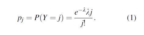
The probability that the count Y generated by a Poisson distribution with Poisson parameter λ is equal to j is

Three models for count data are discussed, namely, (1) the truncated Poisson regression model, (2) the truncated negative binomial regression model, and (3) the Zelterman regression model.

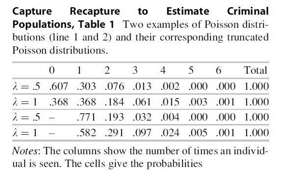
First consider Eq. 1. Two examples of a Poisson distribution are provided in Table 1. In the first example, an individual has a Poisson parameter λ= .5. Then his or her probability to be seen zero times is .607, the probability to be seen once is .303, twice is .076, and so on. These probabilities add up to 1. In the second example, it is assumed that there is an individual with Poisson parameter 1. His or her probability not to be seen is .368, the probability to be seen once is .368, twice is .184, and so on. Note that the individual with Poisson parameter λ=1 has a larger probability to be observed at least once, namely, (1- .368) = .632, whereas this probability for the individual Poisson parameter λ=.5 is only (1- .607) =.393. It follows that the individual with Poisson parameter λ=1 has a larger probability to be seen.

Model 1: The Truncated Poisson Regression Model

In single-register capture-recapture data the observed individuals each have a count larger than zero. Since for the observed individuals the count cannot be zero, these individuals have the so-called truncated Poisson distributions. For the data in the first and second row of Table 1, the truncated distributions for y > 0 are obtained by dividing the probabilities by 1-P(y = 0|λ), that is, for the first example we divide by 1 -.607 = .393 and for the second example we divide by 1- .368 = .632; see rows three and four of Table 1.

As a first step towards developing the truncated Poisson regression model, assume that there are no covariates. This implies the homogeneity assumption, so that only a single Poisson parameter needs to estimated. This Poisson parameter is then used to obtain the probability of not being registered given that the Poisson parameter equals the value λ, as denoted P(y = 0|λ). Using P(y = 0|λ), the part of the population is estimated that we did not see. A small example will illustrate this. Assume that n ¼ 250 individuals are observed with a Poisson parameter for which P(y = 0|λ) = .667.

This would mean that P(y > 0|λ) = .333, that is, only one-third of the population is observed so our n refers to one-third of the population size. The missed part of the population size is (.667/.333) * 250=500. The estimated population size would then be equal to the observed part plus the missed part, that is, N = 250 + 500 = 750. In the statistical literature, this is known as the Horvitz-Thompson estimator of the population size (see Van der Heijden et al. 2003b).

Secondly, the Poisson parameter for individual i is related to the covariate values x_1i , x_2i , … of individual i by a log-linear model, that is,

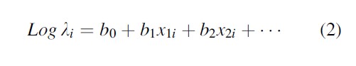
This equation explains the term “regression” in the name “truncated Poisson regression model.” Once the model is estimated and the parameters are known, the Horvitz-Thompson method can be applied on an individual level (see Van der Heijden et al. 2003b). Using the earlier example, for each of the 250 individuals in the data, there is an estimated li-parameter. For each individual i separately, P(y =0|λ_i)/P(y > 0|λ_i) can be calculated, and this yields the number of missed individuals with covariate values identical to individual i. If these numbers of missed individuals over i are summed and 250 is added, the estimated population size is found derived under the truncated Poisson regression model.

Summarizing, the homogeneity assumption is exchanged for a heterogeneity assumption that allows individuals to be different with regard to their covariates. It is important to consider the case where heterogeneity is completely or partly ignored. Van der Heijden et al. (2003a) show that ignoring heterogeneity leads to an estimated population size that is too low. Ignoring heterogeneity may happen if important covariates are not used in Eq. 2.

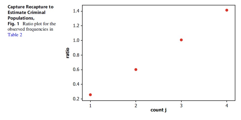
It is possible to investigate whether there is ignored heterogeneity by using a test presented by Gurmu (1991). If this test is significant, then there is evidence for additional heterogeneity (i.e., additional with regard to the heterogeneity that is already taken into account by the covariates), and the estimated population size isto be interpreted as a lower bound for the true population size. Thus, the Gurmu test can be used to investigate the fit of the model. Another way of investigating the validity of the Poisson assumption is the ratio plot (Bohning and Del Rio Vilas 2008). According to the previous section, r_j=( j + 1)p_j+1/p_j=λ, a constant, if the p_j follows a Poisson distribution. Departure from this constant indicated unobserved heterogeneity.

Model 2: The Truncated Negative Binomial Regression Model

The distinction between the truncated negative binomial regression model and the truncated Poisson regression model is that the truncated negative binomial regression model allows for additional heterogeneity of Poisson parameters after the covariates have been taken into account. Equations for the negative binomial model are complicated; see Hilbe (2011) for details.

Cruyff and Van der Heijden (2008) discuss the application of the truncated negative binomial regression model for population size estimation. It turns out that this model is often difficult to fit numerically, in particular when Poisson parameters are small. For details, see Cruyff and Van der Heijden (2008) where this is shown using a simulation study. Unfortunately there are also numerical problems for the example discussed below. For an example of opiate users where fitting the truncated negative binomial regression truncated Poisson regression model did not lead to numerical problems, see Cruyff and Van der Heijden (2008).

Model 3: The Zelterman Regression Model

The Poisson distribution Eq. 1 has the property that, for any j, P( j + 1|λ)/P( j|λ) = λ/( j + 1). This can be rewritten as λ=( j + 1) P( j + 1|λ)/P( j|λ). Zelterman (1988) uses this property to propose local estimators of the Poisson parameter by plugging in observed frequencies f_j of count j for P( j|λ) and P( j + 1|λ). In particular, if the frequencies f₁ and f₂ are plugged in, an estimate of the Poisson parameter

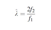
is found, and this estimate of λ can then be used to estimate P(0) =1 – exp(λ) and hence the Zelterman population size estimator N_Z =n/(1- exp(λ)). This estimator is closely related to Chao’s estimator N_C = n + f₁²/2f₂, that is used for similar purposes (Bohning 2010).

Zelterman’s proposal has the advantage that it is robust against violations of the Poisson assumption such as unobserved heterogeneity. Also, when interest goes out to the frequency of the missed count f₀, then it makes sense to use the information that is the most close to f₀, that is, f₁ and f₂, because individuals that make up f₁ and f₂ will be most similar to the individuals that make up f₀. Probably for this reason and because the estimator is easy to understand, Zelterman’s estimator is quite popular in estimates of drug using populations (see, Van Hest et al. 2007).

Recently Bohning and Van der Heijden (2009) generalized the Zelterman estimator so that it can take covariates into account as in Eq. 2. As the Zelterman estimator is a useful competitor of the Poisson estimator if there is heterogeneity of the Poisson parameters, the Zelterman regression model is a useful competitor of the truncated Poisson regression model when the homogeneity assumption of the Poisson parameters (conditional on the covariates) is violated. This follows from the robustness property of the Zelterman estimator.

Model Choice

In the truncated Poisson regression model, the presence of unobserved heterogeneity in the data can be investigated with a test proposed by Gurmu (1991) and ratio plots (Bohning and Del Rio Vilas 2008). If unobserved heterogeneity can be ignored, the truncated Poisson regression model is the model of choice. If unobserved heterogeneity cannot be ignored, the population size estimate given by the truncated Poisson regression model is to be interpreted as a lower bound for the true population size. In this situation, the truncated negative binomial regression model can be tried. However, regularly numerical problems are encountered in the estimation of the model. If there is doubt about the Poisson assumption for individuals having counts higher than 2, then the Zelterman regression model provides a robust estimate.

Example

In the context of domestic violence policy, it is important to have reliable estimates of the scale of the phenomenon. In 2009, a study was conducted to supplement a victim study and perpetrator study (van der Heijden et al. 2009). Here the perpetrator study is reported. cthe prevalence of domestic violence, particularly because so few victims are willing to file charges, which leads to underreporting, that is, the dark number in registers. The aim of the capture-recapture methods used in this study is to estimate the size of the underreporting. Adding up the reporting and underreporting then yields an estimate of the total population of offenders. The estimates have been made using data from incidents that were reported and where charges were filed. The data represent the Netherlands except the police region for The Hague.

The estimates presented have been calculated using the Poisson regression model and the Zelterman regression model. The negative binomial regression model had numerical estimation problems. The estimates are presented for a year ranging from mid-2006 to mid-2007. Distinctions were also drawn as regards specific features of the estimated populations, that is, the sex and age of the individual suspect, the type of violence used, the type of victim of domestic violence, and the ethnic background of the suspect.

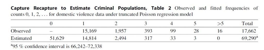
The first line of Table 2 shows the observed distribution of the counts. A total of 17,662 perpetrators are observed in the year ranging from mid-2006 to mid-2007, of whom 15,169 were observed once, 1,957 twice, and so on. The second line of Table 2 shows the fitted values under the truncated Poisson regression model. The estimated population size is 69,290 (confidence interval is 66,242–72,338) of whom 51,629 perpetrators are not found in the police register. The fit of the model is not good, as is revealed by comparing the observed frequency of the counts and the estimated frequency of the counts: The Gurmu test on overdispersion gives a chi-squared distributed test value of 30.04 for 1° of freedom (p < .0001), showing that the departure from the truncated Poisson regression model is significant. Similarly, Fig. 1 shows a ratio plot (Bohning and Del Rio Vilas 2008) where these ratios are monotonically increasing, indicating strong unobserved heterogeneity. For this reason, further results for the truncated Poisson regression model are not presented, but the focus will be on the Zelterman regression model.

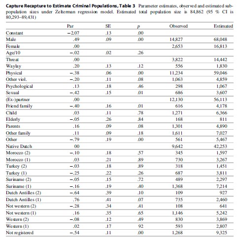
The Zelterman regression model yields a population size estimate of 84,862 (confidence interval is 80,293–89,431). Columns 1–3 of Table 3 provide parameter estimates, standard errors, and p-values for a Wald test. Gender is significant, and the fitted conditional Poisson parameter for males is exp (.49) = 1.63 times as large as the fitted conditional Poisson parameter for females. For type of domestic violence, sexual and physical assaults have a lower fitted Poisson parameter than threat. In comparison to an (ex-) partner, a family friend and “other” have lower fitted Poisson parameters. Ethnic background (first or second generation) is not significant, except for “not registered” in the official register, which are undocumented foreigners, who have a lower fitted Poisson parameter than the native Dutch population.

Columns 4 and 5 of Table 3 provide observed univariate frequencies and fitted frequencies. For example, 14,827 males are found in the police register, and the estimate of the number of males is 68,048; thus, it can be concluded that 14,827/68,048 * 100 =22 % of the male perpetrators is observed. For females, this percentage is 2,653/16,813 * 100=16 %. The other percentage can be derived in an identical way.

Future Directions

It is shown how police records can be used to estimate the size of criminal populations. These estimates can be used to evaluate the effectiveness of the police forces and grant insight into differential arrest rates (Collins and Wilson, 1990) for different groups. Even though the definition of the data is straightforward, however, the data are sometimes contaminated with errors. The reason is that the police does not collect these data for the purpose of conducting statistical analyses, they do so to facilitate the process of apprehending offenders. Therefore, the register is not always as careful as it should be. For example, data cleaning was required to minimize the likelihood of incorrect double counts (i.e., the same apprehension appears twice in the system). Clearly, an incorrect double count incorrectly decreases f_k by 1 and increases f_k+1 by 1, so that there appear to be more recaptures than there actually are. The result is that the estimated zero count is too low. Although careful attention has been devoted to the appearance of incorrect double counts, it is possible that there are still a few in the data.

Conversely, suppose that an individual has been apprehended several times, but this has not been recognized so that this individual has been entered several times as several single persons. This will lead to the result that f₁ is too large whereas f_j with j > 1 is too small, leading to an overestimation.

Apart from problems in the correctness of the data, it may also be that data do not follow the assumptions of the model. This will lead to biased estimates. Above we discussed the problem of positive contagion (leading to estimates that are too low) and negative contagion (leading to estimates that are too high). Another problem discussed above is unobserved heterogeneity, leading to estimates that are too low. It may very well be that unobserved heterogeneity always plays a role when the data are derived from a police registration.

As regards the meaning of our population size estimate, one might wonder what it stands for? Basically, the apprehended individuals can only be generalized to similar individuals who are not apprehended (but who are in principle apprehensible and where charges could be filed). Thus, the population size estimate does not stand for the total number of perpetrators of domestic violence; it stands for the apprehensible ones. The population estimate is still useful, since it represents the number of individuals who pose a threat to society and is thus an indication for the police potential workload.

Capture Recapture to Estimate Criminal Populations, Table 3 Parameter estimates, observed and estimated subpopulation sizes under Zelterman regression model. Estimated total population size is 84,862 (95 % CI is 80,293–89,431)

Bibliography:

1. Bohning D (2010) Some general comparative points on Chao’s and Zelterman’s estimators of the population size. Scand J Stat 37:221–236
2. Bohning D, Del Rio Vilas VJ (2008) Estimating the hidden number of scrapie affected holdings in Great Britain using a simple, truncated count model allowing for heterogeneity. J Agric Biol Environ Stat 13:1–22
3. Bohning D, van der Heijden PGM (2009) A covariate adjustment for zero-truncated approaches to estimating the size of hidden and elusive populations. Ann Appl Stat 3(2):595–610
4. Bouchard M (2007) A capture-recapture model to estimate the size of criminal populations and the risks of detection in a Marijuana cultivation industry. J Quant Criminol 23(3):221–241
5. Bunge J, Fitzpatrick M (1993) Estimating the number of species: a review. J Am Stat Assoc 88:364–373
6. Cameron AC, Trivedi PK (1998) Regression analysis of count data, vol 36, Econometric society monographs no. 30. Cambridge University Press, Cambridge
7. Chao A (1988) Estimating animal abundance with capture frequency data. J Wildl Manag 52:295–300 
8. Collins MF, Wilson RM (1990) Automobile theft : estimating the size of the criminal population. J Quant Criminol 6(4):395–409.
9. Cruyff MJLF, van der Heijden PGM (2008) Point and interval estimation of the population size using a zero-truncated negative Binomial regression model. Biom J 50(6):1035–1050
10. Greene MA, Stollmack S (1981) Estimating the number of criminals. In: Fox JA (ed) Models in quantitative criminology. Academic, New York, pp 1–24
11. Gurmu S (1991) Tests for detecting overdispersion in the positive Poisson regression model. J Bus Econ Stat 9:215–222
12. Hilbe JM (2011) Negative Binomial regression. Cambridge University Press, Cambridge
13. Johnson NL, Kotz S, Kemp AW (1993) Univariate discrete distributions, 2nd edn. Wiley, New York
14. Mascioli F, Rossi C (2008) Capture-recapture methods to estimate prevalence indicators for the evaluation of drug policies. Bull Narc LX(1/2):5–25
15. Rossmo DK, Routledge R (1990) Estimating the size of criminal populations. J Quant Criminol 6:293–314
16. Seber GAF (1982) The estimation of animal abundance, 2nd edn. Griffin, London
17. Van der Heijden PGM, Cruyff MJLF, van Houwelingen HC (2003a) Estimating the size of a criminal population from police registrations using the truncated Poisson regression model. Stat Neerl 57:289–304
18. Van der Heijden PGM, Bustami R, Cruyff MJLF, Engbersen G, van Houwelingen HC (2003b) Point and interval estimation of the truncated Poisson regression model. Stat Model 3:305–322
19. Van der Heijden PGM, Cruyff MJLF, Van Gils GHC (2009) Omvang van huiselijk geweld in Nederland. Ministerie van Justitie, Den Haag, WODC (33 pagina’s)
20. Van Hest NHA, Grant AD, Smit F, Story A, Richardus JH (2007) Estimating infectious diseases incidence: validity of capture–recapture analysis and truncated models for incomplete count data. Epidemiol Infect 136:14–22
21. Wittebrood K, Junger M (2002) Trends in violent crime: a comparison between police statistics and victimization surveys. Soc Indic Res 59:153–173
22. Zelterman D (1988) Robust estimation in truncated discrete distributions with application to capturerecapture experiments. J Stat Plan Inference 18:225–237

See also:

• How to Write a Research Paper
• Research Paper Topics
• Research Paper Examples

Free research papers are not written to satisfy your specific instructions. You can use our professional writing services to buy a custom research paper on any topic and get your high quality paper at affordable price.