Crime Location Choice Research Paper

This sample Crime Location Choice Research Paper is published for educational and informational purposes only. If you need help writing your assignment, please use our research paper writing service and buy a paper on any topic at affordable price. Also check our tips on how to write a research paper, see the lists of criminal justice research paper topics, and browse research paper examples.

Overview

Most behavior of interest to social scientists is choice behavior: actions people commit while they could also have done something else. In geographical and environmental criminology, a new framework has emerged for analyzing individual crime location choice. It is based on the principle of random utility maximization as developed in economics. It integrates the study of spatial crime distributions with journey-to-crime research, and it is used to explain the offender’s choice of where to commit an offense. It allows the analyst to simultaneously assess the role of location attributes and the role of these attributes in relation to offender characteristics, such as their age, ethnicity, gender, criminal experience, and where they live. Initial applications of the model have shown that the decision of where to commit an offense can successfully be described as a function of characteristics of the decision-maker (i.e., the offender), the potential crime target locations, and their interactions, including the distance that separates them. Other applications have established that physical and social barriers inhibit the journey to crime, that railways facilitate the journey to crime, and that offenders are more likely to offend near former anchor points (past homes). New developments in the area of crime location choice include a focus on small spatial units of analysis and the assessment of spatial spillover effects.

Introduction

Many research questions in the social and behavioral sciences, including criminology, deal with understanding and predicting individual choices. Political scientists aim to understand why people vote and what makes them choose a particular political party (Palfrey and Poole 1987). Sociologists want to understand what makes people decide in favor of a particular education, occupation, or marriage partner (Jepsen and Jepsen 2002). In marketing research, understanding and predicting consumer choice is core business (McFadden 1980). Transportation researchers aim to find out what it is that makes commuters choose to travel by bicycle, car, bus, or train (Train 1980). Behavioral ecologists try to find out what influences a nonhuman animal’s choice of where to forage, rest, or reproduce (Krebs and Davies 1993).

Making choices requires agency, that is, the capacity of actors to make decisions. That capacity does not necessarily imply consciousness of the choice process on the part of the decision-maker. Behavioral ecologists, for example, study nonhuman animals’ choices but do not make any assumptions about the mental processes that give rise to these behaviors.

Choice is also a central concern in criminology, victimology, and criminal justice research. The following questions provide some examples. How do judges or juries decide on whether a suspect is guilty or not, and on the type and the severity of a sanction? What makes people decide in favor of perpetrating crime? What makes them select a particular victim?

This research paper is about crime location choice, which addresses the questions where offenders go to commit crime and why they go there instead of somewhere else. The aim of the chapter is to provide a concise but complete discussion of the various issues involved in using the discrete choice framework to understand the spatial decision making of criminals. The remainder of this text first discusses how the issues of crime location choice have been addressed in the literature. It subsequently outlines random utility maximization theory and the discrete choice framework. The section that follows discusses what has been learned substantively from recent applications of the discrete choice framework to crime location choice. The final section discusses pending issues that have yet to be resolved and most of which require additional empirical research.

Different Approaches To Study Crime Location Choice

Crime location choice addresses the questions where offenders commit crime, and why there instead of somewhere else. Before the discrete choice framework was introduced in the geography of crime, there were three separate approaches to the study of crime location choice (Bernasco and Nieuwbeerta 2005). Each of these approaches is characterized by a specific unit of analysis and a specific dependent variable.

The offender-based approach uses either the offender or the offense as the unit of analysis. The dependent variable is the length of the journey to crime, which has always been operationalized as the distance between the home of the perpetrator and the place where the offense was perpetrated. The most basic question answered is the question how far from home offenders perpetrate their offenses. A somewhat more complicated question is whether and how steep the offending intensity decreases with the distance from home. More generally, this question addresses the form of the distance decay function, because it has also been claimed that this distance function is upward sloping near the offender’s home (within a “buffer zone”) and only starts to slope downwardly at greater distance. Still more complicated questions compare the distance between different types of offenders and different types of offenses. Empirical research has shown that most offenders commit their offenses rather close to their homes, that there is distance decay, and that the average distance traveled varies across offense types and across offender types. The theoretical basis of the offender-based approach is small. It starts from the assumption that travel is costly and that for that reason offenders prefer to travel as little as possible to the locations of their offenses. Because this implies that most offenders would perpetrate crime on their doorsteps, and this appears not to be the case, an additional hypothesis has been introduced which states that offenders do not commit crimes close to their own homes for fear of recognition by victims or bystanders.

The offender-based approach is limited for establishing where offenders perpetrate crime and for understanding that choice. It is limited because at any given distance, there are a number of alternative locations (all located on the circle around the offender’s home) that can be selected, and the offender-based model does not provide any further help in understanding the actual location that was chosen. It is also limited because it assumes that distance (and thus travel cost) is the main criterion that determines where offenders perpetrate crime (in addition, offenders would avoid perpetrating very close to their homes for fear of being recognized by victims or bystanders). Thus, the offender-based approach ignores that location choices may be driven by geographic variations in the availability of criminal opportunities (i.e., the presence of suitable victims and targets and the absence of formal and informal guardians) or by characteristics of the offender (e.g., awareness space).

The target-based approach uses potential target locations as units of analysis. The dependent variable is the crime rate or the victimization rate at the target location. This approach actually includes the bulk of studies in geographic criminology in which the crime locations are aggregated to larger areas and related to the characteristics of these aggregated areas, in particular characteristics that signal the presence of suitable victims and targets (e.g., entertainment areas or shopping centers) and the absence of formal and informal guardians (e.g., police presence and likelihood of social control exercised by residents). Thus, while the target-based approach does analyze crime location as a choice outcome, it typically does not consider offender mobility and thus ignores that some areas are vulnerable because they are more accessible to offenders than other areas that are identical in every other respect. For example, a shopping strip may be an ideal place for a late-night street robbery for motivated offenders who live nearby, but if the nearest motivated offender lives 5 miles away, it may not be a suitable location for any offender.

The third approach is the mobility-based approach. The mobility-approach uses pairs of geographical locations as the units of analysis. The dependent variable is the number of crime trips from one of both locations to the other. This approach applies spatial interaction models, also known as gravity models (Haynes and Fotheringham 1984), to model volumes of offender travel within and between the neighborhoods, traffic zones, or other geographic entities in the study area (Elffers et al. 2008; Reynald et al. 2008; Smith 1976). These studies estimate regression models of trips from a particular zone of origin to a particular zone of destination. The variables include the number of observed trips, which is the dependent variable, and crime attractors (services and people that attract criminals from elsewhere to the destination), crime producers (services and people that produce criminal motivation in the origin), and impedance variables. Impedance variables measure the “friction” or obstacles that must be overcome to move from the origin to the destination, including the distance, the travel time, or the cultural or ethnic similarity between the origin and the destination. In the mobility-based approach, distance and other impedance indicators are accounted for as choice criteria: They are independent variables that determine, among other things, how likely an offender from a particular origin location is to perpetrate a crime in a particular destination location. Spatial interaction models analyze aggregate flows of crime, but are not able to appropriately model variation across categories of offenders or among individual offenders. For example, to answer the question whether distance differently affects the crime location choice of juveniles and adults, one would have to estimate separate models for juveniles and adults. This is not a tractable option when the analysis is to include more than just a few categories.

The discrete choice framework constitutes the fourth approach to the issue of crime location choice. The dependent variable in this approach is the choice outcome, that is, which alternative of a countable set of alternative locations does the offender select, and the unit of analysis is the individual decision-maker.

There have thus far been published eight empirical studies that use the discrete choice framework to analyze crime location choice, including Bernasco and Nieuwbeerta (2005); Bernasco (2006); Clare et al. (2009); Bernasco and Block (2009); Bernasco (2010a); Bernasco (2010b); Bernasco and Kooistra (2010); and Bernasco et al. (2012).

Random Utility Maximization And Discrete Choice

In many disciplines, the discrete choice framework (Ben-Akiva and Lerman 1985) has emerged as a powerful and elegant approach to theorize about choice, to statistically model it, and to predict its outcomes. The discrete choice framework is a combination of random utility maximization (RUM) theory and a statistical model of the family of discrete choice models (e.g., conditional logit, multinomial logit, nested logit, and mixed logit models). The models can be used without RUM theory for other purposes than choice modeling, but the major strength of the discrete choice model is that the statistical model is directly derived from RUM theory. Because the theory is a formal (mathematical) theory, its predictions are quite precise and can be tested quantitatively. The intimate link between the theory and the statistical model makes it relatively straightforward to test new elements and conditioning clauses when they are added to the theory. While these features may sound like obvious requirements, most theories in the social sciences are informal and are only loosely linked to the statistical models that are used to test them.

The discrete choice framework is a set of assumptions and methods to model a decision-maker’s choice among a set of alternatives that are mutually exclusive and collectively exhaustive. This means that the decision-maker must select exactly one alternative, and that the alternatives do not overlap, so that by choosing an alternative all other alternatives become unavailable.

Most of the assumptions in the discrete choice framework are based on RUM theory (McFadden 1973). RUM theory is the microeconomic theory of behavior in which a random component is added to the utility function. The random component represents incomplete information on the part of the analyst, not on the part of the decision-maker. By making certain assumptions about the distribution of this random component, the theory is directly linked to a statistical model that allows probabilistic statements to be formulated and tested.

The discrete choice framework was developed in the 1970s by McFadden and others working in the field of travel demand, and the first applications of discrete choice were in the study of travel mode choice (i.e., the choice between train, bus, car, or airplane). Later, the model was also applied to the choice of a travel routes and travel destinations (Ben-Akiva and Lerman 1985).

The discrete choice framework defines four elements of a choice situation (Ben-Akiva and Bierlaire 1999):

1. Decision-makers. The decision-maker is the person or agent that makes a choice.
2. Alternatives. The decision-maker must choose one alternative from the choice set, that is, the set of available alternatives that are mutually exclusive and collectively exhaustive.
3. Attributes. Alternatives have attributes that affect the utility that the decision-maker derives from them when they are chosen. The decision-maker evaluates the utility of all alternatives. The decision-makers themselves can also have attributes that may affect the utility they derive from the alternatives.
4. Decision rule. According to RUM theory, the decision-maker chooses the alternative that maximizes (expected) utility (net gain, profits, satisfaction) when chosen.

In further discussing discrete choice modeling, the notation of Train (2009) is followed. For stylistic reasons and clarity of argument, the decision-maker is referred to as a “he” and the researcher is referred to as a “she.”

A decision-maker, labeled n, must make a choice among the J alternatives in the choice set. Decision-maker n obtains a level of utility (profits, satisfaction) U_ni from alternative i if that alternative is chosen. The decision rule of utility maximization theory asserts that the decision-maker decides in favor of the alternative i if and only if he expects to derive more utility from alternative i than from any other available alternative. Thus, if he decides in favor of alternative i, he must expect to derive less utility from each of the other alternatives.

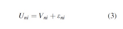
The utilities are assumed to be known by the decision-maker, but not by the researcher. The researcher only observes the actual chosen alternative i, the set of J alternatives, some attributes a_ni of the alternatives, and some attributes d_n of the decision-maker; and she can specify a function V, often called representative utility or systematic utility, that links these observed attributes to the decision-maker’s utility:

The researcher incompletely observes utility, so that generally U_nj≠ V_nj . The utility can be written as the sum of representative utility V_nj and a term ε_nj that captures the factors that determine utility but are not observed by the researcher and that is treated as random.

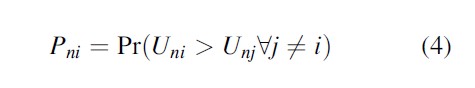
The probability P_ni that decision-maker n chooses alternative i is the probability that the utility associated with choosing i is greater than the utility associated with any other alternative in the choice set:

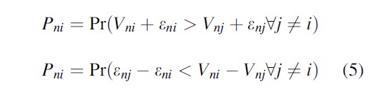
Substituting Eq. 3 in Eq. 4 yields

This is the most general formulation of the discrete choice model. Statistical models that implement this include not only the workhorses of this family, the conditional and the multinomial logit models, as special instances, but also various others, such as nested logit, mixed logit, and multinomial probit. Details of these models are described in Train (2009). All applications of the discrete choice model to crime location choice have thus far used the conditional logit model, which is also referred to as “the (multinomial) logit model with variables that vary over alternatives.” This model assumes that the unobserved utility term ε_ni follows an extreme value type 1 distribution, from which the following formula for the probability that decision-maker n chooses alternative i can be derived.

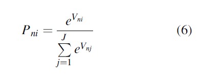
This formula relates the utility derived the alternative that is chosen (the numerator) to the total utility of all alternatives in the choice set (the denominator).

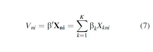
For computational convenience, representative utility V_ni is usually assumed to be linear in the K parameters:

Application Of Discrete Choice Models To Crime Location Choice

The application of discrete choice models to crime location choice implies that the four elements of choice situations are specified. A collection of potential crime locations constitutes the choice set. In most applications of the model thus far, this collection of locations is formed by the set of “neighborhoods” in a single city or region. Thus, the problem addressed can be phrased as “given that an offender will commit an offense in the study area, in which of the neighborhoods in the area will s/he commit it?” Substantive theory is needed to specify what the characteristics of potential targets are that make them attractive to offenders.

Thus far, the discrete spatial choice model has been applied mostly to burglary and to robbery. Studies on burglary include Bernasco and Nieuwbeerta (2005); Bernasco (2006) and Bernasco (Bernasco 2010a) in The Hague, the Netherlands; and Clare, Fernandez, and Morgan (Clare et al. 2009) in Perth, Australia. Bernasco (2010a) and Bernasco and Kooistra (2010) studied commercial robbery in the Netherlands, and Bernasco and Block (2009) and Bernasco et al. (2013) studied street robbery in Chicago, USA. Bernasco (2010b) studied burglary robbery, theft from vehicle, and assault.

Target Characteristics

The discrete choice framework was introduced in criminology by Bernasco and Nieuwbeerta, who used data on 548 burglaries committed by solitary (non-co-offending) offenders in any of the 89 neighborhoods of the city of The Hague, the Netherlands, by offenders who were themselves residents of the city. They argued that burglars would be attracted to targets located near their homes (indicated by distance and by distance to the city center) that were affluent (indicated by property value) and accessible (indicated by percentage single-family dwellings) and where they were least likely to be disturbed by residents or bystanders (indicated by low residential mobility and low ethnic heterogeneity). They found that offenders were attracted to neighborhoods located near their own homes and near the city center, to ethnically mixed neighborhoods, and to neighborhoods with a relatively high percentage of single-family dwellings.

Bernasco (2006) extended this analysis by adding data on co-offender groups, by covering a longer period, and by using factor analysis to group neighborhood characteristics into the sets of variables indicating affluence, physical accessibility, and social disorganization. Only the physical accessibility of neighborhoods was found to significantly increase their odds of being targeted.

The spatial anchor point of offenders structures their choices because it defines the distances that they must overcome to reach target locations. Because offenders live in different locations, the distances between their homes and potential targets vary between potential targets (for the same offender) as well as between offenders (for the same potential target).

An important difference between journey-to-crime research and criminal location choice research is that in the former, variation in distance to crime is the explanandum; distance is the dependent variable. In criminal location choice, distance is part of the explanans; the distance to a potential target is one of the arguments that offenders consider when they decide on where to commit an offense.

Barriers

The findings on burglary in The Hague mentioned above already indicate that distance plays an important role in criminal location choices. Distance is actually a poor measure of the impedance encountered when traveling between two places. Arguably, better measures include monetary cost, travel time, and lack of comfort. Studying 1761 burglaries in 292 suburbs in Perth, Australia, Clare et al. (2009) demonstrated that physical barriers (such as rivers or highways that form obstacles for cross-travel) and connectors (such as public transport lines) affect offenders’ journeys to crime. They also found that the influence of impermeable barriers increases with proximity of these obstacles to the offender’s point of origin.

More abstract barriers to mobility are social in nature. A social barrier deters offenders to commit crime in a potential target area because the potential target area is socially (culturally, ethnically, economically) different from the offender or from the area where the offender lives. A study on Chicago robbers (Bernasco and Block 2009) demonstrated that, controlling for distance from home, offenders displayed a strong tendency to commit robberies in places where the majority of the population was of their own ethnic category. There are two plausible reasons for this finding. First, because birds of a feather flock together, ethnic minorities tend to live together in areas or congregate elsewhere. For this reason, most individuals spend a considerable amount of time in the proximity of their peers, and it is only logical that they commit crime around the places they normally visit. The second reason is that offenders like to disguise their motives and that they may be much less conspicuous in areas where people live who are like they are.

Awareness Space

Crime pattern theory (Brantingham and Brantingham 2008) suggests that for an individual to commit a crime at a place, the place must not only offer criminal opportunities but must also be part of the individual’s awareness space, which is shaped by current and recent routine activities. Recent research utilized the discrete spatial choice model to investigate whether offenders are more likely to target areas near their former residences (Bernasco 2010b; Bernasco and Kooistra 2010). It was demonstrated that offenders were not only likely to offend near their current residence, it was also demonstrated that they were more likely to offend near former homes, especially if they had lived there for a long time and had moved away only recently. This type of idiosyncratic spatial knowledge need not be restricted to offender’s home locations but may include the homes of their friends and family members, as well as other major anchor points such as schools, workplaces, or entertainment and business areas they regularly visit during presumably legal activities.

Offenders must also learn about the criminal opportunities of places where they commit crimes. Indeed, it has been suggested that the phenomena of repeat victimization and near repeat victimization (whereby in the wake of a crime, victimization risk is elevated in the vicinity of the crime site) may be explained by the postulated tendency of offenders to return to their prior targets (Bernasco 2008; Bowers and Johnson 2004). This tendency might be lower for locations where offenders were arrested.

Small Spatial Units Of Analysis

From geography, it is well known that physical and social processes are not constant across spatial scales. The finding that the outcomes of both descriptive and explanatory analyses strongly depend on the size and shape of the spatial units of analysis has been coined the modifiable areal unit problem (or, more neutrally, phenomenon) (Openshaw 1984). As most theories of crime seem to focus on small spatial units, criminologists are urged to collect and analyze data on small spatial units (Weisburd et al. 2009).

In spatial discrete choice, the MAUP has not been given much attention, and studies of location choice, whether in human migration, recreation, or firm location, have typically based the scale decision on convenience and data availability. In crime location research, Bernasco (2010a) and Bernasco et al. (2013) discuss the complexities involved in using small geographical units. The first challenge is mainly computational. Small spatial units of analysis typically imply a large or very large choice set, which may generate computational challenges because the matrix that is used in the maximum likelihood estimation of the parameters has N J records, where N is the number of decision-makers and J is the mean number of alternatives available per decision-maker. Bernasco et al. (2013) demonstrate that in their analyses of street robbery at census block level, they would have to join a set of 12,000 offenders with a set of 25,000 census blocks, yielding a matrix of 300 million records to be included in the maximum likelihood estimation procedures. Fortunately, the coefficients of a conditional logit model can be estimated consistently on a random subset of the alternatives (McFadden 1978). Therefore, sampling from alternatives has become an agreed standard in applications with large numbers of alternatives, including location choice. Guevara (2010) developed methods to sample from alternatives for more complex discrete choice models, such as nested logit.

The second challenge is theoretical. Small spatial units imply that spatial spillover effects may be more salient, especially if spillover effects display strong distance decay. For example, a retail store may not only attract street robbers to the exact location where it is located but also to blocks across the street and around the corner. A robber may follow a customer from a store in one block to a more isolated place in an adjacent block before he attacks, or wait in ambush around the corner. In analyses at higher levels of aggregation, such as census block groups, census tracts, or neighborhoods, such short-distance effects are much weaker because the large majority of the short-distance spillover takes place within the boundaries of the larger geographical units.

Bibliography:

1. Ben-Akiva ME, Bierlaire M (1999) Discrete choice methods and their applications to short term travel decisions. In: Hall RW (ed) Handbook of transportation science. Kluwer, Norwell, MA, pp. 5–34
2. Ben-Akiva ME, Lerman SR (1985) Discrete choice analysis: theory and applications to travel demand. MIT Press, Cambridge, MA
3. Bernasco W (2006) Co-offending and the choice of target areas in burglary. J Invest Psychol Offend Profil 3:139–155
4. Bernasco W (2008) Them again? same offender involvement in repeat and near repeat burglaries. Eur J Criminol 5(4):411–431
5. Bernasco W (2010a) Modeling micro-level crime location choice: application of the discrete choice framework to crime at places. J Quant Criminol 26(1):113–138
6. Bernasco W (2010b) A sentimental journey to crime; effects of residential history on crime location choice. Criminology 48:389–416
7. Bernasco W, Block R (2009) Where offenders choose to attack: a discrete choice model of robberies in Chicago. Criminology 47(1):93–130
8. Bernasco W, Kooistra T (2010) Effects of residential history on commercial robbers’ crime location choices. Eur J Criminol 7(4):251–265
9. Bernasco W, Nieuwbeerta P (2005) How do residential burglars select target areas? a new approach to the analysis of criminal location choice. British J Criminol 45:296–315
10. Bernasco W, Block R, Ruiter S (2013) Go where the money is: modeling street robbers’ location choices. J Econ Geogr 13(1):119–143. doi:10.1093/jeg/lbs005
11. Bowers KJ, Johnson SD (2004) Who commits near repeats? a test of the boost explanation. Western Criminol Rev 5(3):12–24
12. Brantingham PJ, Brantingham PL (2008) Crime pattern theory. In: Wortley R, Mazerolle L, Rombouts S (eds) Environmental criminology and crime analysis. Willan, Cullompton, pp 78–93
13. Clare J, Fernandez J, Morgan F (2009) Formal evaluation of the impact of barriers and connectors on residential Burglars’ macro-level offending location choices. Aust N Z J Criminol 42:139–158
14. Elffers H, Reynald D, Averdijk M, Bernasco W, Block R (2008) Modelling crime flow between neighbourhoods in terms of distance and of intervening opportunities. Crime Prevent Commun Safety 10:85–96
15. Guevara CA (2010) Endogeneity and sampling of alternatives in spatial choice models. PhD Thesis. MIT, Department of Civil and Environmental Engineering, Cambridge, MA
16. Haynes KA, Fotheringham AS (1984) Gravity and spatial interaction models. Sage, Beverly Hills
17. Jepsen L, Jepsen C (2002) An empirical analysis of the matching patterns of same-sex and opposite-sex couples. Demography 39(3):435–453
18. Krebs JR, Davies NB (1993) An introduction to behavioural ecology, 3rd edn. Blackwell, Oxford
19. McFadden D (1973) Conditional logit analysis of qualitative choice behavior. In: Zarembka P (ed) Frontiers in econometrics. Academic Press, New York, NY, pp. 105–142
20. McFadden D (1978) Modeling the choice of residential location. In: Karlkvist A, Lundkvist L, Snikars F, Weibull J (eds) Spatial interaction theory and planning models. North-Holland, Amsterdam, pp 75–96
21. McFadden D (1980) Econometric models for probabilistic choice among products. J Business 53(3): S13–S29
22. Openshaw S (1984) The modifiable areal unit problem. Geo Books, Norwich
23. Palfrey TR, Poole KT (1987) The relationship between information, ideology, and voting behavior. Am J Polit Sci 31(3):511–530
24. Reynald DM, Averdijk M, Elffers H, Bernasco W (2008) Do social barriers affect urban crime trips? the effects of ethnic and economic neighbourhood compositions on the flow of crime in the Hague, the Netherlands. Built Environ 34:21–31
25. Smith TS (1976) Inverse distance variations for the flow of crime in urban areas. Soc Forces 54(4): 802–815
26. Train KE (1980) A structured logit model of auto ownership and mode choice. Rev Econ Stud 47(2): 357–370
27. Train KE (2009) Discrete choice methods with simulation. Cambridge University Press, New York, NY
28. Weisburd D, Bernasco W, Bruinsma GJN (eds) (2009) Putting crime in its place: units of analysis in geographic criminology. Springer, New York

See also:

• How to Write a Research Paper
• Research Paper Topics
• Research Paper Examples

Free research papers are not written to satisfy your specific instructions. You can use our professional writing services to buy a custom research paper on any topic and get your high quality paper at affordable price.