Group-Based Trajectory Models Research Paper

This sample Group-Based Trajectory Models Research Paper is published for educational and informational purposes only. If you need help writing your assignment, please use our research paper writing service and buy a paper on any topic at affordable price. Also check our tips on how to write a research paper, see the lists of criminal justice research paper topics, and browse research paper examples.

Group-based trajectory modeling is a powerful and versatile tool that has been extensively used to study crime over the life course. The method was part of a methodological response to the criminal careers debate but has since greatly expanded in its applications. The current state of the art of group-based trajectory modeling is complex, but worth becoming familiar with so as to recognize the variety of uses to which this tool can be applied. The method has attracted unusually robust criticism for a statistical tool. Researchers should aim to use it and other statistical tools as effectively as possible.

Introduction

Criminologists have long been interested in studying crime as a longitudinal phenomenon. Recent interest stems from vigorous debate surrounding the interpretation of the fact that criminal behavior bears a robust curvilinear relationship with age, quickly ramping up to a peak in the late teen years, and declining thereafter. Part of the criminal careers debate of the 1980s concerned the interpretation of this aggregate relationship. The peak around age 17 may reflect patterns of offending among all offenders, or it may reflect an influx of offenders with relatively short criminal careers around their teen years. In short, the question is whether individual criminal careers resemble the aggregate age-crime curve. This is one of the many questions that group-based trajectory modeling – a general statistical tool for uncovering distinct longitudinal patterns in panel data – can answer.

Group-based trajectory modeling can best be understood in contrast to its alternatives. The most common alternative to group-based trajectory modeling is hierarchical linear modeling, also known as general growth curve modeling. This alternative identifies the average trend over time and quantifies the degree of variation around this average. It is relatively parsimonious because it assumes a specific error distribution around the overall average, typically Gaussian. Group-based trajectory modeling, in contrast, makes no assumptions about the distribution of parameters. Rather, it assumes that the distribution can be approximated by a finite number of support points. Group-based trajectory modeling is related to hierarchical linear modeling in the same way a histogram is related to mean and standard deviation. The mean and standard deviation quickly provide information about the distribution of a variable, but a histogram can provide more detailed information on the shape of the distribution. Both are approximations of a more complex reality. Given a specified number of groups, group-based trajectory modeling attempts to discover a set of longitudinal paths that best represents the raw data. Group-based trajectory modeling is a powerful tool for uncovering distinct longitudinal paths, particularly when significant portions of the population follow a path that is very different from the overall average.

Group-based trajectory modeling is a versatile tool, not limited to revealing distinct longitudinal paths. Once the best group-based trajectory model has been chosen, the researcher may proceed by: (1) describing characteristics of the groups (i.e., characteristics of their growth patterns and covariates); (2) predicting group membership based on preexisting characteristics; (3) evaluating the group-specific effects of time-varying covariates and testing whether such effects vary by group; (4) using groups as independent variables to predict later outcomes; and (5) incorporating measures of group membership as control variables in regression models or propensity score matching protocols. Attesting to its utility and the ease of interpreting its results, although group-based trajectory modeling was developed to answer specific questions posed by the criminal careers model (Nagin and Land 1993), the method has been used to model trajectories of abdominal pain symptoms in pediatric patients (Mulvaney et al. 2006), fungal growth on the forest floor (Koide et al. 2007), and of course, extensive use in the study of longitudinal patterns of criminal activity (Piquero 2008).

This research paper will proceed by first describing some of the theoretical background for the emergence of group-based trajectory modeling. The bulk of the paper will be devoted to describing the state of the art of the method including the basic components of the model, how to choose the number of groups, and several model extensions. Next, it will cover a number of controversies surrounding the method as well as some possibilities for further development.

Background

A central fact of criminology is that a small portion of the population commits a large share of crime. Goring (1913) found that just 3.4 % of the population accounted for about half of all convictions in England. This finding was repeated in a Philadelphia birth cohort: 5 % of the cohort accounted for over half of all police contacts (Wolfgang et al. 1972). This rediscovery of the concentration of offending occurred around the same time that the rehabilitative focus of punishment gave way to rationales of deterrence and incapacitation, creating demand for theoretical accounts and statistical tools that identified high-rate or “chronic” offenders as a distinct group

Alfred Blumstein and colleagues (1986) promoted a criminal careers framework that could be used to describe the volume of crime committed over an individual lifespan, including age of onset, rate of offending, age of termination (desistance), and career length. The criminal careers paradigm suggested that each of these parameters warranted investigation and, possibly, distinct theoretical explanations. It also provided a way to distinguish “career criminals” from others, through their long criminal career length. In opposition to this perspective, Travis Hirschi and Michael Gottfredson (1983) claimed that the criminal careers model did not provide any special insight into age and crime. They claimed the age-crime curve was invariant across social context and no sociological variable was able to account for it. They deemed longitudinal research a waste of resources since the correlates of crime are consistent across age. These two positions formed the basis for the criminal careers debate.

These developments set the stage for a number of theoretical and statistical advances in the 1990s. On the theoretical side, Robert Sampson and John Laub (1993) drew from Glen Elder’s life-course framework (1994) to develop an age-graded theory of informal social control. The life-course framework presents a way of thinking about individual development. Anything that can be measured once can be measured repeatedly, and stringing these measurements together over time creates a trajectory. Embedded within, and providing meaning to these trajectories are life transitions, which, if they redirect the trajectory onto another path, are called turning points. In contrast to Sampson and Laub’s age-graded theory, Moffitt’s (1993) typological theory of antisocial behavior posited that the age-crime curve is made up of two groups with distinct trajectories of antisocial behavior and distinct etiologies.

The criminal careers debate engendered several methodological advances as well. Rowe and colleagues (1990) used Rasch modeling to arbitrate between Hirschi and Gottfredson’s parsimonious latent trait theory and the contention of the criminal careers model that each component of the criminal career may require distinct theoretical explanation. And in 1993, Nagin and Land introduced the group-based trajectory model to address several theoretical puzzles posed by the criminal careers model. This paper modeled longitudinal patterns of individual offending using a finite mixture model of time-varying rates of offending. This established the groundwork for a long line of statistical advances that have profoundly affected the field of criminology.

State Of The Art

Overview

Any phenomenon or characteristic that evolves over age or time in an identifiable population may be an appropriate candidate for group-based trajectory modeling. This tool has the potential to draw out common patterns and help the researcher to make sense of the data. Group-based trajectory modeling produces a parsimonious summary of a complicated distribution of longitudinal developmental trajectories using a finite set of developmental trajectories and their estimated population prevalence. In contrast, hierarchical linear modeling and latent curve analysis summarize this complicated distribution even more parsimoniously, with a single developmental trajectory representing the average, and some characterization of the nature of variation around this average, obtained by imposing fairly strict distributional assumptions.

As opposed to these strict distributional assumptions, group-based trajectory modeling is agnostic on the nature of the distribution of growth parameters. It allows for the possibility for meaningful subgroups within the population that follow distinct developmental paths. The nature and definition of these “subgroups” has fueled a considerable amount of debate. It should be recognized that these groups may only be identified after the developmental paths that define them have already unfolded. That a distinct group is identified by the model does not speak to the issue of prospective identification of the group. Groups must be understood, like simple regression parameters, as useful simplifications and summaries of a complex reality.

Group-based trajectory models can be put to a variety of purposes. Once groups are obtained, description of each group’s developmental paths and antecedents can be very useful. For example, if high-rate stable, medium-rate decreasing, and low-rate offending groups are identified by a particular model, the proportion of each group possessing certain risk variables can provide information of etiological significance. More generally, group membership may be treated as a dependent variable, something to be predicted as accurately as possible. Covariates may be added to the model to assess group-specific effects of certain conditions or life events on the developmental outcome of interest as well as whether these effects statistically differ between groups. Group membership can also be treated as an independent variable in a number of different ways. Variables representing group membership can be used in regression models to parsimoniously control for complicated developmental histories. Groups may also be used as the basis for matching or incorporated into a propensity score matching framework. These and other uses will be described below after first presenting data requirements, parameterization, and practical issues to address in choosing the “correct” model.

Practical Requirements

The group-based trajectory model requires panel data. There must be repeated measurements of a particular dependent variable within some unit of analysis. The unit of analysis depends on the purposes of the researcher and availability of data. To give a sense of the range of questions this method can be applied to, all the following units of analysis would be appropriate and several have been used in published research: person (delinquent, police officer, and academic), residence, street segment, journal article, sports team, gang, prison, terrorist organization, state, country.

There are currently three pieces of software able to estimate group-based trajectory models: MPLUS, the PROC TRAJ add-on to SAS, and the traj add-on for Stata. Estimation specifics in this research paper will refer to PROC TRAJ, the most complete implementation of the method. Using this software, panel data must be structured in wide format: one line for each unit of analysis, with repeated measures of the dependent variable, time, and time-varying covariates represented using distinct variable names.

There are three broad distributional categories permissible for the dependent variable in PROC TRAJ: logit, censored normal, and Poisson. The censored normal distribution is flexible enough to incorporate cases of upper censoring, lower censoring, both, and neither. And the assumptions of the Poisson model can be relaxed using a zero-inflated Poisson parameterization. Categorical dependent variables and other distributions not listed here are not supported in PROC TRAJ.

Balanced panel data is not required. Any unit with one or more observations will be used in estimating the final model. Generally, at least three repeated measures within each unit are preferred to estimate a stable and meaningful model. The independent variable can be represented in units of age, time (years/months/ etc.), or other sequence. It is often desirable to create a meaningful zero value in the independent variable. For example, if estimating trajectories in young adulthood, age can be transformed so that zero represents age 18, and other ages are interpreted relative to age 18. This allows the estimated intercept of each group to quickly be interpreted as the predicted value at age 18. Centering the independent variable and scaling it down by dividing by 10 or 5 also helps the model to converge more readily.

It is worth thinking carefully about the scale of the independent variable, as transforming it can result in very different trajectory models. Consider, for example, the implications of a group-based trajectory model of marijuana use in adolescence with three types of age scales: untransformed age, age relative to the age of onset for marijuana use among those who ever reported using, and age relative to high school dropout among those who ever dropped out. The first scaling of age provides a model that characterizes longitudinal patterns of marijuana use in the population of interest. The second represents desistance/persistence patterns after initial use, and the third reveals marijuana use patterns relative to a potential turning point event.

Finally, it should be noted that the unit of time need not proceed in lock-step for each observation. For example, the model will estimate ideal group-based trajectories from age 14 to 22 even if one-third of the sample is observed only from ages 14 to 18, another third from 16 to 20, and the final third from 18 to 22. The final groups would have to be interpreted with great caution however, since they represent 8-year trajectories when no single individual is observed for more than 4 years.

Estimation

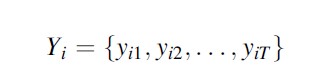
Equations used in this research paper draw heavily from Nagin’s (2005) detailed presentation in Group-Based Modeling of Development. Three subscripts will be used throughout: i refers to the unit of analysis, t to time or age, and j to group. Corresponding to these, N refers to the number of units in the model, T to the number of time periods, and J to the total number of groups in a particular model. The general form of the data used for group-based trajectory models is a set of longitudinal observations for each unit i:

The set of parameters to be estimated for groups 1 through J represents a growth polynomial with respect to the unit of time. The order of the polynomial is specified prior to estimating the model, and can vary across groups. In SAS’s PROC TRAJ implementation of group-based trajectory modeling, the polynomial order of each group’s growth curve can range from 0 to 5. Below, for the sake of example, I present a cubic growth curve for each group j.

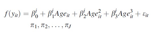
f(y_it) refers to a link function for the outcome of interest. This can either be the censored normal, Poisson, or logit link. In all cases, we are modeling a polynomial on age/time that defines the shape of the trajectory for each group 1 through J. Although the TRAJ procedure lists group membership percents (π_j) among its parameter estimates, it actually estimates J -1 parameters (θ_j) that are used to produce these probabilities. While group membership percents are bounded between 0 and 100 and must sum to 100, theta parameters are completely unbounded. This is useful in estimating the likelihood function. The two sets of parameters are related as follows:

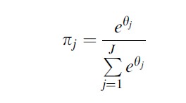
Because J-1 group membership percents define the remaining group membership percent, only J-1 parameters have to be estimated, and θ_j is set to 0, so that it equals 1 when exponentiated. This part of the estimation procedure is the same no matter which type of dependent variable is used.

The goal of estimation is to obtain a set of parameters that maximize P(Y_i), the probability of observing Y_i, the full set of individual developmental trajectories. The likelihood for each individual is obtained by summing the product of the estimated size of each group and the likelihood that the individual belongs to each group, J products for each individual. Estimates are obtained using maximum likelihood estimation with a quasi-Newton algorithm. As a by-product, if the assumptions of the model are sound, it benefits from known properties of maximum likelihood estimates.

Importantly, the model assumes conditional independence: conditional on membership in group j, deviations from the group-specific growth curve at time t is not correlated with deviations from the group-specific growth curve at time t-1. In other words, conditioning on group membership, there is no serial correlation in the residuals. This is a stronger assumption than that made by standard growth curve models (CIA at the individual-level), but growth curve models also assume a multivariate distribution of parameters, which group-based models do not.

The three types of link functions entail additional parameters and modeling decisions. Censored normal models allow for censoring at either the upper or lower bounds and can also accommodate uncensored normal distributions. Lower and upper censoring limits must be provided to model this kind of distribution. If limits are set that are far outside the observed range of data, these limits do not figure heavily in the likelihood function and essentially the uncensored normal distribution is estimated. Otherwise, the model assumes the existence of a latent trait y* that is observed only if the dependent variable is within the upper or lower censoring bounds. When y* is outside the bounds, the observed value, y, is equal to the upper or lower bound. Additionally, censored normal models have the option of estimation of random intercepts and slopes, allowing one to estimate a hierarchical linear model with one group or growth mixture models with multiple groups. Other link functions do not provide this option in PROC TRAJ.

The logit distribution is appropriate for dichotomous outcomes such as arrest, conviction, incarceration, gang membership, high school dropout, etc. Similar to the censored normal distribution, the link function for the logistic distribution assumes the existence of a latent trait y* such that y = 1 if y* > 0 and y = 0 if y* ≤0. If left untransformed, the growth curves from the logistic model are in terms of y* which is the log odds that y = 1.

When the dependent variable is count data such as number of arrests, the Poisson distribution may be appropriate. This distribution requires that the dependent variable take only nonnegative integer values. This type of model was in fact the first presentation of group-based trajectory models because “lambda” in the criminal careers model corresponds directly to lambda in the Poisson model: the rate of offending. Nagin and Land (1993) added a parameter for intermittency that doubles as a way to account for more zero counts than expected from the Poisson distribution. This zero-inflated Poisson (ZIP) model breaks up the probability of a zero count into two components: the probability of a zero count because lambda actually equals zero, and the probability of a zero count by chance when lambda is greater than zero. There are several options for how to specify this model using the “iorder” command in PROC TRAJ. The simplest is to estimate a single parameter for zero inflation across all groups. This can be relaxed in two ways: by estimating group-specific zero-inflation parameters, and by estimating higher order polynomials for the zero-inflation function. Additionally, exposure time can be incorporated into the model to account for different intervals between waves or across units.

Further details on the likelihood functions for these three distributions can be found in Nagin (2005, pp. 28–36).

Choosing The Final Model

PROC TRAJ does not directly reveal the best number of groups. Rather, given a set of data, a model specification, a predetermined number of groups, and starting values (optional), it obtains parameter estimates. There is a danger that these estimates represent local solutions, particularly with very complicated models. The only way to guard against this is to try different sets of starting values to determine if a better solution is obtained. But even the best solution for a specified parameterization and number of groups may not be the best overall solution. A major part of finalizing a group-based trajectory model is choosing the number of groups, tied up with this is the choice of polynomial order and other characteristics of the model.

The model choice set consists of the set of models considered as candidates for the final model. Nagin (2005) recommends a hierarchical decision-making process to reduce the number of models in this set, since it is impossible to try every possibility. The first step is to choose the optimal number of groups. Holding constant other modeling options, vary only the number of groups and assess model adequacy to determine the optimal number of groups. In the second step, specifications for each group are altered until the best solution is obtained, holding constant the number of groups. For example, in Poisson models, should zero inflation be modeled, and if so, should it be general or group-specific and should it be constant or vary over time? The optimal number of groups with general zero inflation may be different from the optimal number of groups with group-specific zero inflation, so this decision point may need to be included in the model choice set at Step 1.

There are a variety of criteria for arbitrating between models to choose the best solution. The most commonly used criterion is the BIC score, based on the log likelihood. The model with the higher BIC score (less negative) is preferred. Given a set of models, the probability that model j is the “correct” model is given by:

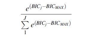
While this may seem to provide a clear guideline for choosing the right model, it is sometimes ignored or downplayed, particularly when the optimal solution according to the BIC score is a very large number of groups. Other quantitative criteria can provide evidence of model adequacy as well.

After model estimation, the probability that each unit belongs to each group can be calculated using the likelihood function. These posterior probabilities are part of the PROC TRAJ output dataset. Each unit’s maximum posterior probability is used to assign units to groups. The maximum certainty for group membership is 1, and the minimum is anything larger than 1/J. The mean posterior probability of group assignment conditional on assignment to that group (AvePP) is indicative of how well that group was identified. Nagin (2005, p. 88) provides a rule of thumb that these average posterior probabilities should be above .7 for each group. However, there is no formal test using this measure that indicates whether a model should be rejected. The minimum group-specific average posterior probability can be compared across models to get a sense of better-performing models. Additionally, an overall average posterior probability can be obtained by averaging every unit’s maximum posterior probability, equivalent to a weighted average of group-specific average posterior probabilities, and a rough correlate of entropy, estimated in MPLUS.

Second, combining group-specific average posterior probabilities and estimated group sizes, one can calculate group-specific odds of correct classification. This essentially compares the ratio of the odds of correctly classifying individuals into group j based on the AvePP value, to the odds of correctly classifying individuals into group j based solely on the estimated proportion of the sample that belongs in group j. It is an odds ratio:

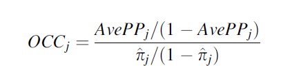
where AvePPj is the group-specific average posterior probability. Nagin’s (2005, pp. 89) rule of thumb is that each OCC should be above 5. Again, however, this is not a formal test, but useful for comparing fit across models.

Nagin also suggests that estimated group probabilities can be compared to the proportion of the sample assigned to the group. Models with more divergent figures are less preferred. No hard limit or even rule of thumb is suggested however, other than “reasonably close correspondence” (2005:89).

PROC TRAJ also has the capability to produce confidence intervals for group membership probabilities and group-specific trajectories. These can also be produced using traditional or parametric bootstrapping. In general, as these confidence intervals widen, models are less preferred.

Finally, solution J + 1 may be rejected because the additional group is not substantively different from any of the groups in the J group solution, for example, when one group is split into two parallel groups. Sometimes a solution is rejected because it identifies an additional group estimated to comprise only a very small fraction of the population, which has limited external validity.

Focusing exclusively on the BIC score can lead to models with little utility. For example, when using a very rich dataset with large N and large T, the upper limit on the number of groups may outstrip their empirical and/or theoretical utility. A more reasonable approach takes into account a variety of model diagnostics to choose the best solution. Unfortunately, there is no ironclad rule for any of these diagnostics. Even the BIC, which seems to offer some certainty to the model choice problem, is highly influenced by the model choice set, and can lead to models which seem to capitalize on random noise. In the end, professional judgment must be exercised in choosing the best model. Taking all diagnostics into consideration, the most defendable and useful model should be retained.

Post-Estimation

As noted in the previous section, after the model is estimated, for each individual and each group, a posterior probability of group membership is estimated. In addition, a categorical variable is created based on posterior probabilities that classifies each unit in a group based on the maximum posterior probability. These are useful in many ways besides model diagnostics. First, they can be used to create group profiles. Second, they can be used as control variables in regression models. Finally, they can be incorporated into matching frameworks.

For each application, there are two options: classify and analyze vs. expected value methods. To illustrate, if we wish to determine the proportion of each group that are male, using the classify-analyze method, we would simply cross-tabulate the categorical group variable with the gender variable. The main shortcoming of the classify and analyze method is that it does not take into account uncertainty in group assignment. When average probability of group membership in a particular group is 75 %, for example, it does not seem advisable to take categorization into the group at face value. Using posterior probabilities takes this uncertainty into account. The expected value method requires a few extra steps to estimate the proportion male in each group. To estimate the proportion of group 1 that is male, calculate the mean for the “male” variable using posterior probabilities for group 1 as a weight. This is repeated for each group. Each person contributes to this group-specific mean proportional to the probability of membership in that group.

The same options are available when incorporating measurements of group membership into regression or matching models. One danger in this type of application, however, is that regardless of which method is chosen, estimation error in group classification is not taken into account. Failing to take this estimation error into account results in biased standard errors. This measurement error can be accounted for using bootstrapping methods.

Model Extensions

Since introducing the PROC TRAJ procedure (Jones et al. 2001), Nagin and colleagues have added a number of modifications and extensions to the model (Haviland et al. 2011; Haviland and Nagin 2005, 2007; Jones and Nagin 2007; Nagin 2005). The discussion here will focus on bootstrapping to obtain confidence intervals, testing equality of coefficients, trajectory covariates, and group membership predictors. Dual trajectory analysis, multitrajectory analysis and incorporating group-based trajectory modeling into matching protocols will be briefly touched upon as well, with reference to other sources for a full treatment.

We can place confidence intervals around any single parameter estimated via group-based trajectory modeling since standard errors are provided for every estimated parameter. However, certain values of interest are functions of multiple estimated parameters. Group membership probabilities are a nonlinear function of J 1 theta parameters and the growth curves themselves are products of polynomials sometimes transformed through a link function or otherwise modified through extra parameters of the Poisson and censored normal specifications. There are several approaches that can be taken to address this problem and place confidence intervals around these estimates.

A typical approach to bootstrapping would create a large number (500, for example) of samples by resampling from the original dataset with replacement, and reestimate the trajectory model on each of the samples to generate a distribution of parameters, group membership proportions, and/or levels of each group’s developmental trajectory to obtain a confidence interval free of distributional assumptions. While this approach is possible using PROC TRAJ, it can be very time intensive. Further, it’s not clear that trajectory groups have consistent meaning across bootstrap samples.

Nagin (2005) suggests using parametric bootstrapping to obtain confidence intervals. Instead of resampling and reestimating the model, parametric bootstrapping simulates the exercise by using the means of the parameter estimates and the variance/covariance matrix. These are taken as values defining a multivariate normal distribution, for which a large number of draws are estimated, and then confidence intervals are obtained the same way they usually are, by appropriate percentile ranks. Because the multivariate normal distribution is well defined, taking even 10,000 replications is much easier than even 500 replications via traditional bootstrapping.

Jones and Nagin (2007) propose a third alternative for generating confidence intervals around growth curves. They introduced a “ci95m” option in PROC TRAJ that provides 95 % confidence intervals around growth curves using Taylor polynomial expansion to approximate the standard errors of combinations of parameters. These confidence intervals can be plotted using the “%trajplotnew” macro. Regardless of how confidence intervals are obtained, they are useful for establishing the precision of a group-based trajectory model. Distinct groups become less interesting if their confidence intervals overlap. Similarly, we change our assessment of a 5 % high-rate offending group if we learn that the confidence interval for the group’s size ranges from 1 % to 20 % versus 4 % to 6 %.

Jones and Nagin (2007) also introduced an important macro add-on for PROC TRAJ that allows one to easily conduct Wald tests for equality of coefficients (%trajtest). This can be used to test equality of growth parameters across groups and has a number of important applications in combination with other extensions of PROC TRAJ described below.

The life-course paradigm organizes the study of human development around longitudinal trajectories, life transitions, and turning points. If a life transition shifts an individual’s developmental trajectory onto a new path, it is a turning point. This suggests a counterfactual type of analysis, answering the question of what would have happened for individuals in situations which they did not experience. Group trajectories, because they represent a group of individuals that are similar with respect to their developmental path and related covariates, provide an important source of plausible counterfactuals to test for these kinds of effects. Group-specific trajectories can easily be generalized to accommodate m time-varying covariates (x₁ through x_m):

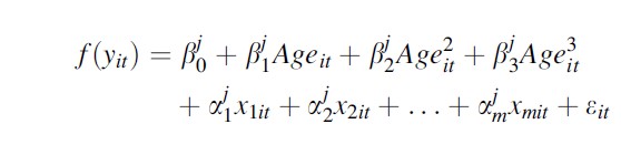
Trajectory covariates can test a wide range of hypotheses from life-course criminology. The specific interpretation of these covariates depends on how they are entered into the model. The simplest strategy is to enter a series of dummy variables reflecting being in a particular life state such as being married, in a gang, employed, etc. This results in group-specific estimates that are easy to interpret, but does not capture the dynamic element of turning points. It does allow for an easy test of whether the effects of that life state depend on group membership, using the %trajtest macro. It assumes constant effects over time/age and over years in the state.

If marriage is introduced in this manner, it imposes an assumption that the effect of marriage depends neither on when a person gets married nor length of marriage. A more flexible method consistent with the life-course paradigm would enter a dummy variable for being in a particular state, age interacted with this dummy variable, as well as a counter variable for years in the state. This would allow the effect of marriage to vary according to when one gets married and to increase or decay depending on how long one stays married.

While posterior probabilities and group membership categories can be used to create group risk profiles, these profiles are of limited use because of error estimates biased due to lack of incorporation of group estimation error. But these risk variables can be incorporated directly into trajectory models, allowing all parameters to be estimated at the same time and with correct standard errors.

The trajectory model changes in several important ways when risk variables are incorporated into it. The shape of the trajectories in the optimal solution may change, and posterior probabilities depend not only on levels of the dependent variable but also on risk variables. Group membership probabilities are estimated conditional on a set of risk variables (x₁ through x_r, for r risk variables). Multiple thetas are estimated for each group. These are used to generate predicted group probabilities for specified sets of risk variables.

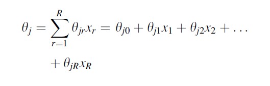
With risk variables, the intercept theta estimates can be used to calculate group membership probabilities when all risk variables are equal to zero. If all risk variables are centered at their means before estimating the trajectory model, then the intercepts would represent theta estimates at the average. The differential impact of risk variables on group membership probabilities can be tested using the %trajtest macro, and confidence intervals around theta estimates or group membership probabilities for specific sets of risk variables can be calculated using bootstrapping.

When more than one dependent variable is of interest, either because of comorbidity of developmental trajectories, heterotypic continuity or a developmental predictor of a developmental outcome, a couple options are available in PROC TRAJ. Dual trajectory analysis (Jones and Nagin 2007; Nagin 2005, Chap. 8) is a very flexible extension of standard trajectory analysis. The basic requirement is that two dependent variables are meaningfully linked via the unit of analysis. Each unit should have repeated observations for both dependent variables. The dependent variables need not be distributed the same way, need not be measured at the same time nor have the same number of measurements, and the estimated number of groups need not be identical. The two dependent variables are linked through a shared variance-covariance matrix and a set of group membership probabilities for one series that are conditional on group membership in the other series. These allow the full set of unconditional, conditional, and joint group membership probabilities to be estimated. Conditional group membership predictors can be included as well.

When more than two dependent variables are of interest, the parameter space for extending the dual trajectory analysis quickly becomes unwieldy. But when the focus is on only two or three dependent variables, multitrajectory modeling is available in PROC TRAJ using the “MULTGROUPS” option (Jones and Nagin 2007). This type of model is constrained in that no cross-classification is estimated across dependent variable types. Instead, each group is defined by a set of trajectories across two or three dependent variables. This simplification greatly reduces the number of parameters that need to be estimated while still providing a rich portrayal of group heterogeneity. As with dual trajectory analysis, the distribution of the dependent variables, the number of observations (T) need not match, and the timeframe need not overlap. The main restriction is that the number of groups must be the same, and of course no cross-classification is estimated.

Recent work incorporates group-based trajectory modeling into a matching framework (Haviland and Nagin 2005, 2007). The basic insight of this work is that developmental histories can serve as important proxies for more complicated processes, and matching within developmental history group serves to balance numerous characteristics – not only the dependent variable of the trajectory model, but numerous related developmental trajectories and risk variables correlated with these trajectories. Haviland and Nagin (2005, p. 4) think of these groups as “latent strata in the data.” Of course, the power of this method depends quite a bit on the extent to which the developmental history being modeled is linked to the selection process for the treatment of interest.

If treatment is random conditional on group membership, this method can provide a convincing measure of turning point effects, where estimated effects are group specific, but can be aggregated through a weighted average to obtain population average effects. Haviland and Nagin’s method establishes developmental paths preceding potential turning points. Within each path, there are two possibilities, one might experience the turning point event, or not. Those individuals within the developmental group who do not experience the turning point event serve as natural counterfactuals for those that do. Assessing differences longitudinally after the turning point event allows us to see whether differences between the two groups emerge, and whether those differences increase, remain stable, or decay over time. To the extent that they persist, evidence for the existence of a turning point is shown. Life-course research also suggests that the response to a turning point event may depend on prior developmental histories. This method allows one to explicitly test that hypothesis. To the extent that groups do not balance important treatment predictors, the group-based trajectory model can be incorporated into a more general propensity score framework, either with propensity score models embedded within each trajectory group, or posterior probabilities of group membership incorporated into a single propensity score model.

Controversies

Group-based trajectory modeling has attracted an unusual amount of criticism of a surprisingly harsh tone. Objections to group-based trajectory models center around the meaning of “group” and the relative merits of alternative statistical models.

Since the concentration of offending was publicized by Wolfgang and colleagues (1972), the search for the high-rate offending group before they engage in the bulk of their crimes has taken up a great deal of resources. In fact, reliably prospectively identifying the chronic offender has been something of a white whale of criminology for decades. Blumstein and Moitra (1980) showed that retrospective identification of groups in Wolfgang et al. did not hold up prospectively, so that the “chronic offender” label was not useful for selective incapacitation of “career criminals.” More recently, Sampson and Laub (2005) have shown that although retrospective offending groups can be identified in their Boston data, even very rich sets of theoretically based predictors cannot reliably distinguish between the groups prospectively. The central point is that even though high-rate offending “groups” can be identified retrospectively either through simple decision rules as in Wolfgang et al. (1972), or through more statistically sophisticated methods such as group-based trajectory models, clustering or other finite mixture models, prospectively, for policy and theoretical purposes, these “groups” do not exist. This is not to say that these groups have no significance, but that their identification in a group-based trajectory model is just the starting point. If the researcher wants to make the case that a specific group is important, that argument must be grounded in theory (Brame et al. 2012) and there must be some demonstration that the group exists outside a single group-based trajectory model.

Critics of this method either over-interpret the significance of groups or imply that because of the nature of the model, other less sophisticated researchers will reify the groups. But of course, the search for the “chronic offender” that Blumstein and Moitra (1980) debunked demonstrated that sophisticated models are not needed in order for reification of a high-rate offender typology to occur.

Many critiques of group-based trajectory modeling are premised on the notion that another statistical tool is superior. Generally speaking, there are three options for summarizing longitudinal developmental patterns: group-based trajectory models, hierarchical linear models, and growth mixture models. Each of these models simplifies a more complex reality in a different way. The differences boil down to how heterogeneity in developmental patterns is characterized. Hierarchical linear models characterize heterogeneity as a jointly normal distribution of parameters centered around the overall average. Group-based models characterize heterogeneity using a mixture of a finite number of growth curves that are support points of a complex distribution. Growth mixture models combine the two strategies, modeling jointly normal distributions of parameters around each group’s average trajectory. Arbitrating between these choices depends on the nature of the research problem and the purposes of the analysis. Nagin (2005) points to complexity of the continuous distribution as an important guide when choosing between group-based and hierarchical linear models.

Future Directions

To date, although group-based trajectory modeling has been extensively employed in the criminological literature, its uses have usually been limited to descriptive exercises. More sophisticated applications such as Haviland and Nagin’s matching method and correct modeling of standard errors using some form of bootstrapping have been less often employed. It is hoped that future work using the method will realize its full capabilities.

Despite the lack of uptake of these more sophisticated features, further development of the model has the potential to greatly benefit the field. The range of dependent variable distributions, although sufficient for most applications in criminology, could be expanded. For example, multinomial, categorical, and quantile group-based trajectories could have immediate applications. Advances such as multitrajectory modeling could be generalized to any number of dependent variables, allowing for complex characterizations of developmental history typologies and perhaps an even stronger basis for identifying latent strata in the data. And the problem of local solutions could be tackled and better understood by incorporating an automated start value algorithm, which is currently offered in the MPLUS implementation of the model.

Conclusion

Group-based trajectory modeling is a powerful tool that can be put to a very wide variety of uses alongside hierarchical and growth mixture models. Through careful, thoughtful use, it can test a number of important theoretical hypotheses (Brame et al. 2012).

Bibliography:

1. Blumstein A, Moitra S (1980) The identification of “career criminals” form “chronic offenders” in a cohort. Law Policy 2:321–334
2. Blumstein A, Cohen J, Roth JA, Visher C (eds) (1986) Criminal careers and “career criminals”. volume 1. National Academy Press, Washington, DC
3. Brame R, Paternoster R, Piquero AR (2012) Thoughts on the analysis of group-based developmental trajectories in criminology. Justice Q 29:469–490
4. Goring C (1913) The English convict. His Majesty’s Printing Office, London
5. Haviland AM, Nagin DS (2005) Causal inferences with group based trajectory models. Psychometrika 70:557–578
6. Haviland AM, Nagin DS (2007) Using groupbased trajectory modeling in conjunction with propensity scores to improve balance. J Exp Criminol 3:65–82
7. Haviland AM, Jones BL, Nagin DS (2011) Group-based trajectory modeling extended to account for nonrandom participant attrition. Soc Methods Res 40:367–390
8. Hipp JR, Bauer DJ (2006) Local solutions in the estimation of growth mixture models. Psychol Methods 11:36–53
9. Hirschi T, Gottfredson MD (1983) Age and the explanation of crime. Am J Soc 89:552–584
10. Jones BL, Nagin DS (2007) Advances in group-based trajectory modeling and a SAS procedure for estimating them. Soc Methods Res 35:542–571
11. Jones BL, Nagin DS, Roeder K (2001) A SAS procedure based on mixture models for estimating developmental trajectories. Soc Methods Res 29:374–393
12. Jr Elder GH (1994) Time, human agency, and social change: perspectives on the life course. Soc Psychol Q 57:4–15
13. Koide RT, Shumway DL, Bing X, Sharda JN (2007) On temporal partitioning of a community of ectomycorrhizal fungi. New Phytol 174:420–429
14. Laub JH, Sampson RJ (2005) Shared beginnings, divergent lives: delinquent boys to age 70. Harvard University Press, Boston
15. Mulvaney S, Warren Lambert E, Garber J, Walker LS (2006) Trajectories of symptoms and impairment for pediatric patients with functional abdominal pain: a 5-year longitudinal study. J Am Acad Child Adolesc Psychiatry 45:737–744
16. Nagin DS (2005) Group-based modeling of development. Harvard University Press, Cambridge, MA
17. Nagin DS, Land KC (1993) Age, criminal careers, and population heterogeneity: specification and estimation of a nonparametric, mixed Poisson model. Criminology 31:327–362
18. Piquero AR (2008) Taking stock of developmental trajectories of criminal activity over the life course. In: Liberman A (ed) The long view of crime: a synthesis of longitudinal research. Springer, New York
19. Sampson RJ, Laub JH (1993) Crime in the making: pathways and turning points through life. Harvard University Press, Boston
20. Wolfgang ME, Figlio RM, Sellin T (1972) Delinquency in a birth cohort. University of Chicago Press, Chicago

See also:

• How to Write a Research Paper
• Research Paper Topics
• Research Paper Examples

Free research papers are not written to satisfy your specific instructions. You can use our professional writing services to buy a custom research paper on any topic and get your high quality paper at affordable price.