Inferential Crime Mapping Research Paper

This sample Inferential Crime Mapping Research Paper is published for educational and informational purposes only. If you need help writing your assignment, please use our research paper writing service and buy a paper on any topic at affordable price. Also check our tips on how to write a research paper, see the lists of criminal justice research paper topics, and browse research paper examples.

Crime mapping has become extremely popular as an analytic technique in the last 20 years and is arguably the default mode of analysis for law enforcement officers. A more detailed treatment can be found at Chainey and Ratcliffe (2005).

The purpose of this research paper is to outline a number of ways that the practice of crime mapping could be improved. Many analysts receive incomplete training in spatial analysis, and most in-house training consists of how to interrogate the various crime databases with very little or no time spent on theories of crime and criminality nor how to conduct analysis (generating and testing hypotheses, drawing inferences). There is currently a paucity of guidance on how to construct the analysis endeavor with notable exceptions being Ekblom (1988), Weisel (2003), and Hirschfield (2005). Two recent examples of hypothesis testing in crime analysis have been provided by Townsley, Mann, and Garrett (2011) and Chainey (2012).

A lack of analytical training has grave consequences for the quality of intelligence products. Without guiding principles, it is very easy to “uncover” patterns and relationships in data that are spurious. For instance, Diana Duyser, of Florida, found an image of the Virgin Mary in her grilled cheese sandwich (BBC 2004). While it is possible that this and other images are demonstrations of divinity, another explanation is pareidolia, when vague and random stimuli are perceived as clear and important. Sagan (1995) speculated that pareidolia may be a side effect of evolution as facial recognition is instinctive in humans.

A more germane example to law enforcement is the birthday problem: how many people would have to be in a room before you are confident that two people present share the same birthday? The answer is 23 for a 50 % chance and 57 to be 99 % confident (Saperstein 1972). Most people find this a surprisingly small number for a small initial probability. Yet intelligence analysts regularly construct social network graphs of individuals of interest trying to linking these to other individuals of interest. But the birthday problem demonstrates it is reasonably easy to establish connections once sufficient individuals are in the group. What no analyst can say, or even thinks to ask, is what they would expect to find for someone who has no connection to the criminal underworld.

Operational law enforcement relies on analysts that interpret the criminal environment, produce intelligence products that influence decision-makers, who then take action to impact the criminal environment (Ratcliffe 2008). The realities of operational law enforcement are that decisions need to be made with incomplete data, in imperfect conditions, and under significant time pressure. The intention of this research paper is to offer broad guidelines to analysts on how to better construct hypothesis testing and draw inferences. Without a systematic approach to assessing evidence, there seems a high chance of misinterpretation. This research paper contains five fundamental principles of analysis, influenced heavily by statistical reasoning and inspired by Dawid (2005). Statistical reasoning is the focus here because it is science of making decisions in the face of uncertainty.

Statistical Principle 1: Frequencies Versus Rates

A basic tenet of scientific enquiry is analysis using rates instead of frequencies. A rate is a frequency adjusted for the underlying population at risk. They are considered superior to count data because frequencies do not reflect the different exposure “at-risk” populations face. For instance, more crime is committed in the USA compared to the UK, but when the population of each country is controlled for, the USA has much a lower crime rate than the UK for nearly all crime classifications except murder (Langan and Farrington 1998).

In the context of crime, there are two underlying problems with the application of rates for measurement. First, the frequency of crime has tangible meaning for practitioners. For instance, while the property crime rate for the City of Omaha, Nebraska, is roughly the same as the City of Philadelphia, Pennsylvania (3730.7 and 3708.2 property crimes per hundred thousand population, respectively), their very different populations (464,628 versus 1,558,378, respectively) mean that the City of Philadelphia hosts roughly 3.3 the number of property crimes of the City of Omaha (FBI 2011). No one would suggest that both jurisdictions require the same level of resources for operational purposes, yet the crime levels, once the at-risk population is accounted for, are practically identical.

Second, locating valid denominators for crime rates is challenging because the population at risk is far from clear for many crime types. Criminal justice researchers are most familiar with crime incidence, the number of crimes per hundred thousand population, but residential population is not appropriate for certain crime types. Central business districts, night-time entertainment precincts, sporting arenas, and tourist locations have very low residential populations but have the potential to host large volumes of crime.

A related issue is the temporal relevance of the denominator. Vehicle crime has almost no connection with residential population; Rengert (1997), for instance, shows that the distribution of vehicle crime in Philadelphia can be explained by the time of day and not by residential population. At a larger scale, seasonal variation in crime rates (McDowall et al. 2011; Baumer and Wright 1996) suggests different limitations with conventional indicators of the population at risk.

A review by Harries (1981) found three main ways of reporting crime: (1) frequencies, (2) population-based rates, and (3) risk-related opportunity. As to be expected with any list of alternative measures, each has advantages over the others in particular circumstances. Frequencies make sense in an operational context or for highly focused, local research efforts. Population-based rates, where the residential population is used as the denominator, are suitable for interpersonal crimes at areal units around city size (Pyle and Hanten 1974). Units of analysis smaller than this do not typically have residential populations estimated with sufficient precision.

Opportunity-based rates use the population at risk as the denominator in rate calculation. For instance, to compute a commercial burglary rate the number of retail outlets could be used as the denominator. While there may be a strong correlation between residential population and shops, the scope of a crime problem is heavily influenced by the available targets in an area. As noted by Phillips (1973, p. 224, emphasis added) [] “[o]ne thing is certain, true risk-related crime rates reveal a far different pattern than had been previously described and are a necessary starting point in any geographic research concerning crime in urban areas.”

Opportunity-based rates are difficult to calculate due to the wide variety of alternate denominators that could be chosen for any given crime type. Moreover, there are considerable logistical difficulties in compiling these indicators. To estimate vehicle crime rates, Boggs (1965) used the amount of parking space as a proxy for the number untended cars, the latter an impractical measure for routine crime analysis.

Another issue with opportunity-based crime rates is they largely represent the number of available targets, and R. V. Clarke (1984) argues convincingly that targets are not created equal and a simple count of targets does not correspond to opportunity. A number of crucial factors may operate to alter a given target’s suitability, such as ease of exploitation, attractiveness, and defended perceptions. Moreover, available targets express different level of vulnerability over the course of a day (see J. H. Ratcliffe (2006) for a theoretic and empirical justification).

One of the methodological problems facing most police organizations is that information systems record crime incidents as point level information, with precision measured in meters when accurate property parcel databases are used. Rate calculation requires some level of aggregation to cruder levels of resolution (e.g., streets, beats, communities). For example, the following figure is taken from the Safe as Houses project in Enfield, UK (Enfield 2011), a finalist in the Herman Goldstein Problem-Oriented Policing Awards in 2011. Problem analysis showed concentrations in particular sections of the borough, one of which is depicted in Fig. 1. It shows frequencies of burglaries for electoral wards around the A10 motorway. The analysts inferred that because the crime count is much higher around the A10 that these properties face an increased risk of victimization, consistent with the empirical literature that more accessible streets host more crime because they are exposed to offenders at a greater rate than less accessible streets (Beavon et al. 1994; Johnson and Bowers 2010).

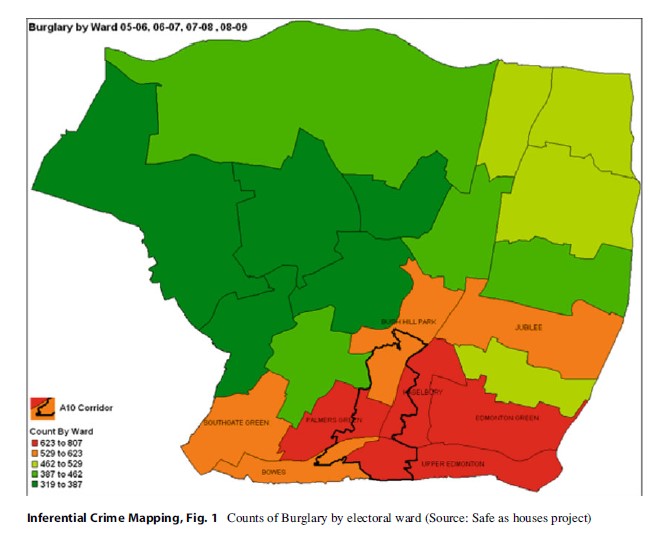
There are two issues with this figure and the inference drawn. First, it is impossible to gage the underlying population at risk. The difference in crime counts may simply be a reflection that there are many more residential dwellings in the electoral wards around the A10. Second, the Modifiable Area Unit Problem (MAUP) (Openshaw 1983) may be operating. MAUP is a pernicious problem in spatial analysis, occurring when arbitrary spatial units (such as administrative boundaries) are used to aggregate data. Different boundaries, especially when they have no connection with the phenomenon of interest, produce contrasting spatial patterns. Gerrymandering is a powerful illustration of the impact of the MAUP.

This project was selected because it is unusually thorough and is clearly the product of tremendous effort. The fact that it was a finalist is evidence that this represents an atypically nuanced and empirical treatment of a crime problem. The point is that if basic problems can be identified in an exemplar case study, then how prevalent are they in less rigorous analytic products?

There are a number of recent examples of opportunity-based rates in crime mapping. Chainey and Desyllas (2008) compute the pedestrian population in various London streets to generate assault rates per hour per street segment. This revealed that some areas that have a notorious reputation were actually some of the safest seats in London. A similar type of analysis, although used for a completely different purpose, was conducted by Kurland and Kautt (2011). They used street population data to quantify the level of crime around football stadiums in the UK. Ambient pedestrian population measures from Land-Scan (http:/www.ornl.govscilandscan) were used to estimate population at risk on certain days and times.

Statistical Principle 2: Making Comparisons

The next foundational principle of statistical reasoning is making comparisons. Comparative information features prominently in statistical reasoning, from baseline measurements, to the use of control groups, even to inferential testing (the null hypothesis provides an expectation and this is compared with reality; test statistics quantify the extent of differences in this comparison).

Crime figures, used in isolation, are meaningless without reference to a comparison area or some baseline crime level because they cannot be put into perspective. The newspaper headline declaring “Over 40 robberies this year” implies this is a high volume of incidents, but without reference to other statistics it is difficult to interpret the claim with confidence.

A common comparison choice is to use an area as its own “control”; that is, the area’s history serves as a baseline indicator to assess current performance. This is analogous to a repeated measures design, a type of analysis where a cohort is measured on more than one occasion. The advantages of this design are beyond the scope of this research paper, but it has a number of highly desirable inferential features. The main point is that each observation in the sample is compared with itself to detect a change.

Even if a baseline period was established, a confounding issue is regression to the mean, a tendency for an area with an extreme score at one point in time to have a score much closer to the average on the next measurement period. This is a frequent problem in crime prevention where areas selected for attention because they contain a hot spot. When regression to the mean occurs, it is natural for analysts, decision-makers, and researchers to credit an intervention or tactical responses with curbing or suppressing a rising crime trend, after all a reduction was expected as a result of the tactics employed.

Another popular method of conducting comparisons is to use a comparison group. Pawson and Tilley (1997) provide a persuasive note of caution about their value. The argument is that interventions trigger mechanisms that fire in particular contexts. An intervention is designed explicitly for the particular area in question, yet comparison groups are conventionally identified through matching demographic and socioeconomic indicators, not the context. Two areas may be strikingly similar with respect to aggregate census indicators yet have neighborhood dynamics which would render some interventions infeasible.

The importance of making comparisons is reasonably straightforward, and spatial researchers could easily argue that crime maps actually possess an inherent comparison; crime maps contain simultaneous displays of hot and cold spots. However, this does not entirely capture the statistical principle of making comparisons. A map of crime density displays the where of crime, serving simply as a form of analytical triage indicating where attention should be placed. What next? What should law enforcement attempt to do to the criminal environment to change to reduce the level of crime?

The overarching goal of analysis is to make some causal claim or inference. For example, poor place management leads to more assaults is a causal statement that links the presence or absence of place management with varying degree of assaults. Statisticians would formally label poor place management as an independent variable (sometimes explanatory variable) and assaults as the dependent variable. The volume of assaults is said to “depend” on the amount of place management.

In order to make comparisons, analysts need to demonstrate that the spatial pattern of some independent variable is closely aligned with the observed pattern of crime incidence (the dependent variable). Explanatory factors are rarely a feature of crime mapping products (Eck (1997) provides a rare example of crime mapping that fully incorporates theory).

Statistical Principle 3: Retrospective Versus Prospective

Many risk factors are expressed in terms of a retrospective proportion. This is where the prevalence of risk factors among an interest group (victims or offenders, say) is computed. For instance, a study claims that 80 % of sexual assaults take place on the public transport system. The inference drawn is that there is a high chance of victimization if you use public transport. Notice the shift in emphasis between the data and the inference:

• If victimized, there is a high chance of using public transport (data).
• If using public transport, there is a high chance of being victimized (inference).

It is clear there is a difference between these two statements, yet the vagaries of language make it easy to slip between these two distinct meanings. In statistical parlance, each of these statements is a conditional probability of the form, P(A | B) where the probability of outcome A is conditioned on (or constrained by) the necessary occurrence of B. The conditioning event is always located to the right the “|” symbol.

To clarify, a conditional probability is the probability of event A occurring if B also occurs. A simple form of inference is to compare conditional probabilities with simple probabilities, probabilities of a single event – P(A). The extent of difference between simple and conditional probabilities implies an association between A and B. Of course, this just establishes an association, a type of correlation. This is not the same as claiming that A causes B. In order to do this, the analyst needs to demonstrate (1) the temporal sequencing such that a change in B corresponds to a change in A and (2) dismissing competing explanations. The statements can be expressed in formal statistical terms:

• P(PT | V) the probability of public transport use among victims (data)
• P(V | PT) the probability of victimization among public transport users (inference)

These are two entirely different quantities as demonstrated in the following table.

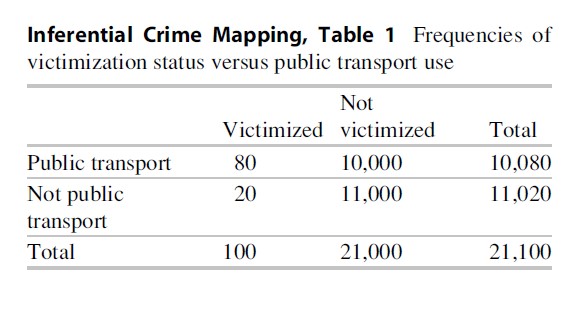
It is reasonably straightforward to see that of those people who have been sexually assaulted, 80 % (=80,100) were on public transport. It is equally easy to see that for those people who are not sexually assaulted, 48 % (1,000,021,000) used public transport. These suggest an association between victimization and public transport and are consistent with the first two statistical principles – these quantities are rates and comparisons are being made. Importantly, these quantities relate to the likelihood of public transport patronage for victims and non-victims.

Unfortunately there is a further problem with retrospective proportions as they give an inflated sense of the association. The statistic of immediate interest is the likelihood of victimization among public transport users, the prospective proportion. Referring to Table 1, this prospective proportion is .8 % (=8,010,080). The corresponding percentage for nonpublic transport users is .2 % (2,011,000).

Two points should be obvious. First, prospective proportions maintain the same order as their retrospective counterparts. The association between public transport and victimization is preserved such that the presence of public transport does correspond to a higher victimization rate regardless of which type of proportion is used.

Second, the prospective proportions are considerably smaller in magnitude than the retrospective proportions, yet this is of more relevance. The problem is that retrospective proportions create the impression that there is a high chance of crime, yet they quantify the likelihood of observing the risk factor (public transport), not the outcome measure (crime). The prospective proportion is about the likelihood of crime.

Analysts need to be aware that due to the nature of crime, they will invariably be calculating retrospective proportions about crime risk factors. Following individuals prospectively when the event of interest is rare or has low frequencies is time and cost prohibitive. Instead, it is far simpler to take a sample of individuals that have observed the event of interest and examine their antecedent attributes. These are useful but are limited in their inferential insight. Retrospective proportions will point to associations, but the strength of those relationships is not immediately apparent. As seen in the example here, quoting the retrospective proportion implies that victimization is a near certain occurrence if one was foolish enough to use public transport, yet the prospective proportion seems far, far less alarming.

Statistical Principle 4: Selection Bias

This principle reflects the observation that forces influencing the data collection process shape the results of analysis performed on the data. Selection bias occurs when the process of data collection is non-probabilistic. Celebrated examples of selection bias occur in election polling (Squire 1988; Jowell et al. 1993), leading to inaccurate estimates. Increased use of mobile telephones has further compromised telephone polling, with some households having no landline telephone (Keeter 2006).

Selection bias occurs naturally whenever secondary data analysis is performed. This is a well-recognized problem that accompanies all crime analysis. Maguire (2012) writes in the most recent volume of the Oxford Handbook of Criminology of the differences between victimization surveys and official statistics. Commonplace problems – which offences are reported to police, which get recorded by police – act as filters on the information contained in police information system. The cumulative impacts of these and other recording practices are to skew the crime analyst’s depiction of the criminal environment.

With respect to spatial analysis, there are a number of additional pressures on crime data which may further impact selection bias. J. H. Ratcliffe (2001) writes that the process of geocoding, where spatial reference information is assigned to crime event data, could be faulty due to a number of reasons:

• Out of date cadastral map. Cadastral maps are a register of property parcels in a region. They contain validated, government information about spaces. Cadastral information is very useful for geocoding because street addresses can be linked to known land survey information. However, if this information is out of date, such as buildings have been demolished or property parcels have been combined to form larger spatial units, then it is likely that geocoding will be inaccurate if applied to new spatial units that do not appear in the cadastral map.
• Abbreviations and misspellings. Reported crime may be misspelled, mispronounced, or incomplete in some way, such as an absent street number. Under these conditions, geocoding is unlikely to operate correctly, with addresses either failing to find a match or being mismatched to a separate address.
• Local name variations. Certain places develop a nickname or local business name which may not appear in an address database. Geocoding works on known street addresses, which victims may be oblivious of if they are not an employee or local community member. Tourists are often unaware of street addresses of locations they visit, for instance.
• Address duplication. Certain street names are more common than others and, without ancillary suburb or community level information, can easily be placed in another area.
• Nonexistent addresses. Mistakes in data entry can easily modify the reported address so it is positioned out of range of a street segment. For example, 18 Baker Street can be transcribed as 80 Baker Street.
• Non-addresses. Public space is a notoriously difficult to record and/or capture reliably, and there are a number of locations that may not exist in a cadastral map. For instance, public parks may be defined as a polygon of the geographic extent of the park, yet it is difficult to see how any geocoding engine could distinguish where any incident would have occurred. In most cases, anything occurring in the park is “recorded” at a single location for the entire park such as the centroid of the polygon. Bichler and Balchak (2007) show that address matching procedures in the major mapping software applications are prone to distinctive systematic biases in geocoding errors. J. H. Ratcliffe (2001) demonstrates geocoding inaccuracy of between 5 % and 7 % in a dataset where crimes recorded in an incorrect census tract. This level of inaccuracy seriously undermines any spatial analysis performed at all but the crudest of spatial resolutions.

Statistical Principle 5: Simpson’s Paradox

This principle operates when patterns of rates (or proportions) calculated for an entire sample are not consistent for patterns for subgroups of the data. The paradox is a reflection of changing denominators in crime rates and is a result of only relying on proportions or rates as indicators of activity. The contradiction is that Simpson’s Paradox directly contradicts the first principle listed here. Of course, it really underlines the importance that counts and rates need to be incorporated in analysis.

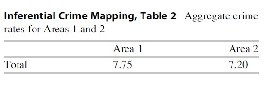
To illustrate, consider you were responsible for two policing jurisdictions and the crime rates for three priority crimes were as listed in the following table. Being a diligent analyst you compute rates for each of these based on appropriate denominators. It appears that Area 2 is safer than Area 1, in aggregate (Table 2).

Given that Area 2 has the lower crime rate, it would be worth considering what examples of best practice might be transferred to Area 1. Exploring differences across different crime types will aid in identifying areas worth targeting. However, examining each crime type shows that Area 2 has a higher crime rate for all crimes (Table 3).

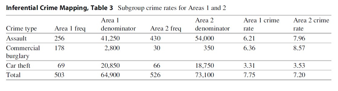
The reason this apparently contradictory result occurs is due to differences in the denominator that are used to compute the rates as well as a reliance on only rates to assess relative risk. Examining either the “at-risk” populations or the volume of crime would indicate that the two areas have certain fundamental differences which may need to be incorporated in addition to considering crime rates.

This principle is a reflection that variation is unequally distributed among locations and facilities. Aggregate summaries of crime may not be representative at finer levels of resolution. For instance, Brantingham, Dyreson, and Brantingham (1976) provide a nice depiction of the changing nature of crime patterns viewed at different levels of resolution. National patterns differ greatly from regional patterns which are different still from local patterns.

Even the use of sophisticated modeling techniques does not protect research findings from Simpson’s Paradox. Roncek and Maier (1991) found a positive association between the presence of licensed venues and the volume of crime. They use the technique which estimated the average impact of a bar on an average block. However, the frequency of crimes for individual bars shows that the effect of an “average” bar is atypical and that only a minority of bars account for the majority of alcohol-related crime and instabilities (Eck et al. 2007).

Spatial Principles

The five principles outlined pertain to any quantitative analysis. Spatial data and analyses in particular have a number of unique attributes that need to be controlled for, or at least accounted, in order to provide valid findings. These are mentioned briefly here:

• Modifiable area unit problem (Openshaw 1983). This is an issue that occurs when point level information is aggregated to areal spatial units that are defined by arbitrary administrative boundaries. If the boundaries used do not have a clear alignment with the social phenomena in question, it is possible to generate a depiction of crime that is a reflection of the properties of the boundaries. For instance, a hot spot located close to the border between two police beats will appear diluted if the hot spot is bisected by the border of the police beats. Using a different set of spatial units will probably “undercover” this hot spot.
• Spatial autocorrelation. Tobler’s first law of geography states observations that located close tend to be more similar to each other than far observations (Tobler 1987). This is a problem because it suggests that observations that are proximate are not statistically independent. This is a fundamental assumption of many inferential techniques in hypothesis testing. Michael Townsley (2009) provides a list of techniques useful for incorporating spatial autocorrelation in analysis or investigating whether is present.

Conclusion

The purpose of this research paper has been to outline fundamental principles of statistical reasoning with a view to informing operational crime analysts about better ways of approaching pattern detection. The target audience for this research paper may very well ask exactly how should analysis be conducted in order to observe these principles. There are three main strategies:

1. Be more scientific. The discipline of crime science has emerged in the last decade and is focused on ways to make crime harder to commit and how to catch offenders quicker. It emphasizes that practitioners should think more scientifically, generate hypotheses, test them, and collect high-quality data. One of the missing gaps in this literature is an acknowledgement of how to conduct analysis in a scientific way. Recent studies by M. Townsley, Mann, and Garrett (2011) and Chainey (2012) put forward methods and examples of how to carry this out.
2. Employ more sophisticated methods. One of the advantages of more sophisticated statistical techniques is that many of the principles of statistical reasoning are “baked in,” especially regression models. There needs to be much more investment in increasing the training of analysts so that they can exploit well-developed quantitative methodologies. If crime science is analogous to medical science, at present there is no analogue to epidemiology in the study of crime.
3. Be more focused and use crime theories. Analysts need to define their problem precisely, restricting their attention to a finite set of behaviors to analyze. For instance, analysts should not study assaults by criminal classification (aggravated assaults, grievous bodily harm, assault with a weapon); rather, they should focus on the relationship between the parties involved. These will range typically from spouses or partners (domestic violence), road rage incidents, school pupils, bar patrons and door staff, and strangers. Each of these assault types has a unique opportunity structure and probably different space-time signatures. Failure to partition each of these discrete problems means that aspects of each are consolidated into an aggregate uninformative blob.

Bibliography:

1. Baumer E, Wright R (1996) Crime seasonality and serious scholarship: a comment on Farrell and Pease. Brit J Criminol 36:579–581
2. BBC (2004) Woman ‘blessed by the holy toast’. http://news.bbc.co.uk/2/hi/americas/4019295.stm
3. Beavon DJK, Brantingham PL, Brantingham PJ (1994) The influence of street networks on the patterning of property offenses. In: Ronald V, Clarke G (eds) Crime prevention studies, vol 2. Criminal Justice Press, Monsey
4. Bichler G, Balchak S (2007) Address matching bias: ignorance is not bliss. Pol Int J Police Strat Manag 30:32–60
5. Boggs SL (1965) Urban crime patterns. Am Sociol Rev 30:899–908
6. Brantingham PJ, Dyreson DA, Brantingham PL (1976) Crime seen through a cone of resolution. Am Behav Sci 20:261–273
7. Chainey S (2012) Improving the explanatory content of analysis products using hypothesis testing. Policing 6 (2):108-121
8. Chainey S, Desyllas J (2008) Modelling pedestrian movement to measure on-street crime risk. In: Liu L, Eck JE (eds) Artificial crime analysis systems: using computer simulations and geographic information systems. Idea Group, Hershey, pp 71–91
9. Chainey S, Ratcliffe JH (2005) GIS and crime mapping. Wiley, Chichester
10. Clarke RV (1984) Opportunity-based crime rates: the difficulties of further refinement. Brit J Criminol 24:74–83
11. Dawid PA (2005) Probability and proof. In: Anderson TJ, Schum DA, Twining WL (eds) Analysis of evidence. Cambridge University Press, Cambridge
12. Eck JE (1997) What do those dots mean? Mapping theories with data. In: Weisburd DL, McEwen T (eds) Crime mapping and crime prevention, vol 8. Criminal Justice Press, Monsey, pp 377–406
13. Eck JE, Ronald V, Clarke G, Guerette RT (2007) Risky facilities: crime concentration in homogeneous sets of establishments and facilities. In: Farrell G, Bowers KJ, Johnson SD, Townsley M (eds) Imagination for crime prevention: essays in honour of Ken Pease, vol 21. Criminal Justice Press, Monsey, pp 225–264
14. Ekblom P (1988) Getting the best out of crime analysis. Crime prevention unit. Home Office, London
15. FBI (2011) Crime in the United States by metropolitan statistical area, 2010 (Table 6).”
16. Harries KD (1981) Alternative denominators in conventional crime rates. In: Brantingham PJ, Brantingham PL (eds) Environmental criminology. Sage, Beverly Hills, pp 147–165
17. Hirschfield A (2005) Analysis for intervention. In: Tilley N (ed) Handbook of crime prevention and community safety. Willan, Cullompton, pp 629–673
18. Johnson SD, Bowers KJ (2010) Permeability and crime risk: are cul-de-sacs safer? J Quant Criminol 26:89–111
19. Jowell R, Hedges B, Lynn P, Farrant G, Heath A (1993) Review: the 1992 British election: the failure of the polls. Public Opin Q 57:238–263
20. Keeter S (2006) The impact of cell phone noncoverage bias on polling in the 2004 presidential election. Public Opin Q 70:88–98
21. Kurland J, Kautt P (2011) The event effect: demonstrating the impact of denominator selection on ‘floor’ and ‘ceiling’ crime rate estimates in the context of public events. In: Morina AD (ed) Crime rates, types and hot-spots. Nova, Hauppauge, pp 115–144
22. Langan PA, Farrington DP (1998) Crime and justice in the United States and in England and Wales, 1981–96. US Department of Justice, Office of Justice Programs, Bureau of Justice Statistics
23. London Borough of Enfield (2011) Safe as houses: reducing domestic burglary project. Finalist, Goldstein POP Awards, http://www.popcenter.org/library/awards/ goldstein/2011/11-09(F).pdf
24. Maguire M (2012) Crime data and statistics. In: Maguire M, Morgan R, Reiner R (eds) The Oxford handbook of criminology. Oxford University Press, Oxford, pp 241–301
25. McDowall D, Loftin C, Pate M (2011) Seasonal cycles in crime, and their variability. J Quant Criminol 28(3):389–410
26. Openshaw S (1983) The modifiable areal unit problem. Geo Books, Norwich
27. Pawson R, Tilley N (1997) Realistic evaluation. Sage, New York
28. Phillips PD (1973) Risk-related crime rates and crime patterns. Proc Assoc Am Geog 5:221–224
29. Pyle GF, Hanten EW (1974) The spatial dynamics of crime. Research Paper Series. Department of Geography, University of Chicago, Chicago
30. Ratcliffe JH (2001) On the accuracy of tiger-type geocoded address data in relation to cadastral and census areal units. Int J Geog Inform Sci 15:473–485
31. Ratcliffe JH (2006) A temporal constraint theory to explain opportunity-based spatial offending patterns. J Res Crime Del 43:261
32. Ratcliffe JH (2008) Intelligence-led policing. Willan,Cullompton
33. Rengert GF (1997) Auto theft in Central Philadelphia. In: Homel R (ed) Policing for prevention: reducing crime, public intoxication and injury. Criminal Justice Press, Monsey, pp 199–220
34. Roncek DW, Maier PA (1991) Bars, blocks, and crimes revisited: linking the theory of routine activities to the empiricism of hot spots. Criminology 29:725–753
35. Sagan C (1995) The demon-haunted world: science as a candle in the dark. Random House, New York
36. Saperstein B (1972) The generalized birthday problem. J Am Stat Assoc 67(338):425–428
37. Squire P (1988) Why the 1936 literary digest poll failed. Public Opin Q 52:125–133
38. Tobler WR (1987) Experiments in migration mapping by computer. Cartogr Geog Inform Sci 14:155–163
39. Townsley M (2009) Spatial autocorrelation and impacts on criminology. Geog Anal 41:450–459
40. Townsley M, Mann M, Garrett K (2011) The missing link of crime analysis: a systematic approach to testing competing hypotheses. Policing 5:158–171
41. Weisel DL (2003) The sequence of analysis in solving problems. In: Knutsson J (ed) Problem oriented policing: from innovation to mainstream, vol 15. Criminal Justice Press, Monsey, pp 115–146

See also:

• How to Write a Research Paper
• Research Paper Topics
• Research Paper Examples

Free research papers are not written to satisfy your specific instructions. You can use our professional writing services to buy a custom research paper on any topic and get your high quality paper at affordable price.