Measuring Crime Specializations and Concentrations Research Paper

This sample Measuring Crime Specializations and Concentrations Research Paper is published for educational and informational purposes only. If you need help writing your assignment, please use our research paper writing service and buy a paper on any topic at affordable price. Also check our tips on how to write a research paper, see the lists of criminal justice research paper topics, and browse research paper examples.

Research on crime at places is a rapidly growing literature. Though Eck and Weisburd (1995) coined the term “crime at places,” the starting point of this literature was Sherman et al. (1989) in a microspatial analysis of predatory crime in Minneapolis. This research area finds that calls for police service are highly concentrated in very few places: 50 % of calls for police service are generated from 5 % of street segments (or less), particularly when one considers detailed crime classifications (Sherman et al. 1989; Andresen and Malleson 2011). Moreover, research has shown that spatial crime patterns at microspatial units of analysis vary significantly across crime classifications (Andresen and Malleson 2011). Because of this consistency, Weisburd et al. (2012) put forth the Law of Crime Concentrations.

One implication from this research is that opportunity surfaces for different crimes, though they may overlap, are different – the opportunity surface for a crime is the distribution of targets across the landscape. From the theoretical perspective of environmental criminology, this statement is rather trivial: routine activity theory (Cohen and Felson 1979) posits that crime occurs when a motivated offender and suitable target converge in time in space without the presence of a guardian – this convergence occurs at a place. In the geometric theory of crime (Brantingham and Brantingham 1981), crimes occur at discrete locations (places) within the boundaries of our activity spaces. And in rational choice theory (Clarke and Cornish 1985), crimes are the result of context-specific choices that consider the immediate environment (places) within which a crime occurs. Even beyond these various theories, one only needs to consider where targets are located for different crime classifications: commercial burglary and robbery only occur in commercial districts, and residential burglary only occurs in residential districts, for example. Needless to say, whether one considers theory or the most straightforward aspects of our (built) environment, crime specializes at places.

Crime specialization is different from crime concentration. We have long known that crime concentrates in places, and those places vary by crime classification (Quetelet 1842). Specialization does not necessarily occur in the same places as concentration. Crime concentration is typically measured using crime rates (a crime count scaled by a population at risk); by the nature of this calculation, places with high crime rates (high degrees of concentration) have greater levels of crime per capita than places with low crime rates. Crime specialization, however, may occur in places with low levels of crime per capita – specialization may be defined relative to the entire study area. As such, the form of measurement necessary must consider the crime mix in some form. Location quotients provide an excellent example of this form of crime measurement.

Location Quotients: The State Of The Art

The location quotient is a geographic measure of specialization. One of the benefits of the location quotient is that it only relies on data for the phenomenon in question; if a researcher is analyzing crime only, crime data are needed. This proves useful because measures of concentration (crime rates) have a number of methodological issues that emerge because they require other data (Andresen 2006). Of course, the location quotient still suffers from all the problems associated with crime reporting issues and the dark figure of crime, a concern in quantitative-based studies of crime dating back to at least the early nineteenth century (Bulwer 1836). Regardless, the location quotient is calculated as follows:

where C_in is the count of crime i in subregion n, C_tn is the count of all crimes in subregion n, and N is the total number of subregions. In this context, the location quotient is a ratio of the percentage of a particular type of crime in a subregion relative to the percentage of all crime in that same region. If the location quotient is equal to one, the subregion has a proportional share of a particular crime; if the location quotient is greater than one, the subregion has a disproportionately larger share of a particular crime; and if the location quotient is less than one, the subregion has a disproportionately smaller share of a particular crime. Specifically, if a subregion has a location quotient of 1.20, that subregion has 20 % more of that crime than expected given the percentage of that crime in the region as a whole – that subregion then “specializes” in that crime classification. Miller et al. (1991) provide the following classifications that are useful for interpreting the location quotient: very underrepresented areas, 0≤LQ≤0.70; moderately underrepresented areas, 0.70 < LQ ≤0.90; average represented areas, 0.90 < LQ ≤ 1.10; moderately overrepresented areas, 1.10 < LQ≤1.30; and very overrepresented areas, LQ > 1.30.

Brantingham and Brantingham (1993, 1995, 1998) introduced the location quotient into criminological research in the early 1990s, but its adoption as a standard criminological measurement has been slow. With a primary concern for violent crime, Brantingham and Brantingham (1993, 1995, 1998) use the location quotient to measure the crime mix and specialization within a municipality; they compare the location quotient results to those for crime counts and crime rates. The larger municipalities in their study, not surprisingly, had the highest counts. However, after controlling for population size, the large municipalities no longer ranked at the top of the list, but now towards the bottom of the list. Smaller hinterland municipalities topped the list when using crime rates. Yet another ranking emerged with the location quotient: some municipalities with high crime rates also have high location quotients, but there are also a number of municipalities that have low crime rates with high location quotients. Consequently, there are municipalities that have low risk of crime in general (low crime rates), but specialize in violent crimes.

Though this phenomenon of specializing in a particular crime when the risk of crime is rather low is interesting in itself (and the focus of this research paper), this property may allow one to investigate a curious result that emerges when considering crime rates. In the context of illegal drugs in the United States, Rengert (1996) expects the north central region of the United States to have the greatest proportions of marijuana crimes (of all drug-related crimes) because of a lack of a coastline and its agricultural base – heroin and cocaine are expected to be greatest in coastal regions because of a greater need to transport the drugs internationally. However, Rengert (1996) finds that the spatial pattern of marijuana crimes effectively follows the same spatial pattern as heroin and cocaine when using calculations based on the crime rate: the north central region of the United States is ranked last. However, when Rengert (1996) uses the location quotient to consider crime specialization, the pattern reversed. Therefore, the other regions of the United States had greater volumes and corresponding rates of marijuana crimes than the north central region, but if one were to commit a drug crime in the north central region, it is most likely to be related to marijuana.

Curiously, aside from one study that uses the location quotient as a component in a composite index, its use in criminology is absent for 10 years. In this more recent research, McCord and Ratcliffe (2007) use the location quotient to measure crime intensity across neighborhoods and find that drug markets tend to cluster close to pawnshops, drinking establishments, and mass transit stations. Andresen (2007) performs an inferential analysis (spatial regression) using the location quotient as a dependent variable and finds that if independent variables are interpreted as attractors of a particular crime, it performs well in a predictive manner. Ratcliffe and Rengert (2008) use the location quotient to identify areas that have greater intensities of shootings, relative to the city as a whole. Andresen (2009) investigates the phenomenon of crime rates in Canadian provinces increasing as one moves east to west – crime rates in the territories are even higher than in the western provinces. Andresen (2009) uses the location quotient to show that simply because all crime rates are greatest in the west does not mean that western provinces specialize in all crimes. In fact, crime specialization is present in all provinces for at least two crime classifications in each province. This analysis vividly shows that crime concentration (crime rates) does not necessarily imply crime specialization. Most recently, Block et al. (2012) use the location quotient in the context of automotive theft in the United States. They find that states and counties that contain or are near heavily trafficked borders and ports specialize in automotive theft; Block et al. (2012) speculate that this is an indication for the presence of a “theft for export” problem in these areas. Moreover, these are not always areas that have high rates of automotive theft.

Clearly, the location quotient’s popularity in spatial crime analysis has increased in recent years. However, its general lack of adoption in criminological research is somewhat surprising because it allows for the measurement of crime specialization. Regardless, there are a number of other measures of specialization that may prove to be useful to criminologists. Some of these measures are already being used within the criminological literature in other (nonspatial) contexts, whereas others are used in geography and economics that prove insightful in a criminological context. To illustrate these, calls for service data are used below to show their utility.

An Empirical Example Of Measuring Specialization

In order to perform the calculations below (crime rates, location quotients, and other measures of specialization), crime data are necessary. All crime data are for 2001 in the City of Vancouver, British Columbia, Canada. The areal unit of analysis is the dissemination area (DA). These units are defined by Statistics Canada and are similar to the census block groups in the United States Census. There are 990 DAs in Vancouver in 2001. The calculations below consider both property crime and violent crime classifications: assault, burglary, robbery, sexual assault, theft, theft of vehicle, and theft from vehicle – homicide is excluded because there are so few cases, twelve homicides for the entire year. Property crime counts and percentages dominate violent crime counts and percentages, as expected; property crimes account for just over 83 % of the 60 427 incidents included in the calculations below.

All crime data used below come from the Vancouver Police Department’s Calls for Service Database (VPD-CFS Database) generated by its computer-aided dispatch system. Though the VPD-CFS Database is actually a proxy for actual crime data because not all calls for service represent actual crimes, the primary advantage of the VPD-CFS Database is this raw form – these data are not dependent on a criminal charge, though few calls for service are subsequently unfounded by the VPD. The geocoding success rate for these data was 93 %; though computer algorithms for geocoding have limitations that may lead to concerns over accuracy (Ratcliffe 2001), the current success rate is well above the minimum acceptable success rate of 85 % (Ratcliffe 2004).

Mapping The Location Quotient

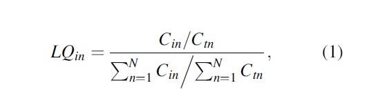
Though the discussion regarding the location quotient above may be instructive to show the utility of its calculation, an example using burglary highlights the distinction between concentration and specialization. The burglary rate per 1,000 households in Vancouver (2001) is shown in Fig. 1a. It should be clear to the reader that burglary has its greatest concentrations in the eastern section of the central business district, the downtown eastside, as well as in a number of other areas that correspond to commercial land use, mixed land use, and arterial roadways; burglary is also in greater concentrations within the eastern side of the city – the eastern side of Vancouver has lower income levels than the western side of Vancouver, on average.

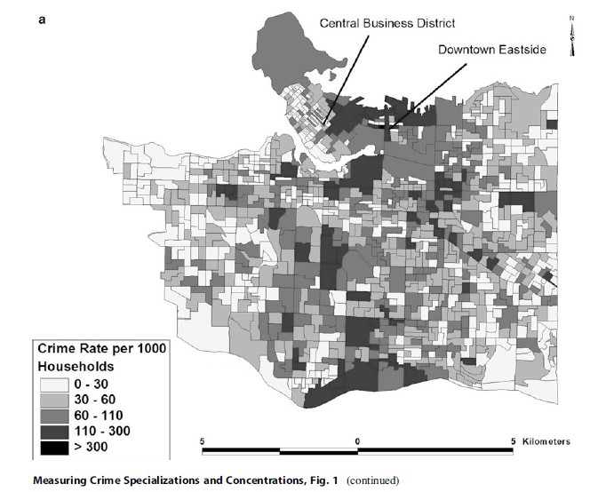
The spatial pattern of the location quotient for burglary (Fig. 1b), however, has a very different spatial pattern. Though there are areas throughout Vancouver that exhibit specialization, by far specialization occurs within the western side of Vancouver. This region of the city contains some of the wealthiest neighborhoods of Vancouver that all have relatively low levels of concentration in burglary. If one were to analyze other crime classifications in Vancouver, the results are not as stark as with burglary, but this example shows that where crimes are concentrated are not necessarily the same places in which specialization occurs.

Alternative Measures Of Specialization

The first alternative measure considered here is a normalized version of the location quotient, normalized such that its values range from zero to unity. Though the algebra provides the same value, this normalized location quotient is based on the Balassa (1965) Index and is commonly used in the international trade literature (De Benedictis et al. 2009):

The calculation of the normalized location quotient, referred to as the relative Gini in the literature (De Benedictis et al. 2009), is calculated as follows:

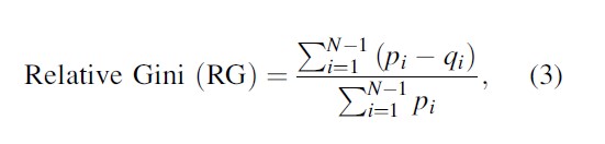
where p_i is the share of crime i within the study area as a whole (Vancouver in the current context) and q_i is the share of crime i within the subregion (dissemination area in the current context). In order to perform this calculation, all q_i are ranked according to their values with the top value being excluded. All values of q_i are ranked for the purposes of identifying the top value so it can be excluded from the calculation. This is done in order for the index to have a range from zero to unity. If q_N is included and there is total specialization (that must occur in that classification, by definition), the index takes on a value of zero. Clearly this makes the index of little value if this situation is a possibility. In the case of total specialization in a subregion, q_N=1 and the index value is equal to zero. As such, if the research wishes to have total specialization have a value of unity, the calculation may easily be modified to be 1 – RG

Though the location quotient has now been normalized, this measure is not without limitations. First, the natural interpretation of the location quotient has been lost: a value of 1.20 indicates that crime i specializes in a subregion by 20 %, relative to the study area as a whole. Such statements can no longer be made. Second, the normalized location quotient is not specific to a crime classification. Rather, it is a measure of specialization, generally speaking.

Another index that uses the location quotient in its calculation is one of the many variants of the Theil (1967) Index. The Theil Index is a measure of relative specialization:

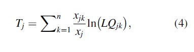
where x_jk is the count of crime k in subregion j, x_j is the count of all crime in subregion j, ln() is the natural logarithm operator, and LQ_jk is the location quotient for crime k in subregion j, as calculated above in Eq. 1. When T_j = 0 there is no specialization and T_j has an upper bound of ln(z), where z is the number of basic units (crime classifications); in the current context, the upper bound of T_j = ln(7) = 1.94.

The Theil Index, though instructive, also has its limitations. As with the normalized location quotient, though the Theil Index is calculated for each subregion, it is a general measure of specialization and does not provide information regarding which type of crime classification specialization occurs in a particular subregion. Also, the Theil Index is undefined if the share of crime k in a subregion is zero because the location quotient is then zero and the natural logarithm of zero is not defined. Of course, one may use a small number in place of zero, but this is dependent on the concerns of the study. If knowing that none of a particular crime occurred in a subregion is critical information, a different measurement of specialization would be more important. This increasingly becomes a problem in the context of crime as the spatial unit of analysis becomes smaller. As shown in the crime at places literature, many places consistently have no crime (Sherman et al. 1989; Andresen and Malleson 2011).

The Diversity Index is the next specialization measure to consider here. The Diversity Index is calculated as follows:

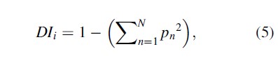
where p_n is the percentage of offenses in category n and i refers to the subregions. This index has been used in the criminological literature as a measure of offender specialization (Johnson et al. 2009) – this index may only be calculated using the latter summation term, depending on whether or not the researcher wants the value of zero or unity to indicate specialization. Though criminologists often point to other criminological or sociological research as its source, this index is a variant of the Herfindahl-Hirschman Index in economics that measures industrial concentration – see Herfindahl (1950) and Hirschman (1945).

In its original formulation,

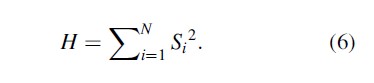
H ranges from 1/N to unity, with N being the number of firms in an industry and S_i being the market share of firm i; in the current context, the number of crime classifications is under consideration. In order to have the index range from zero to unity, the following normalized H (H*) has been proposed:

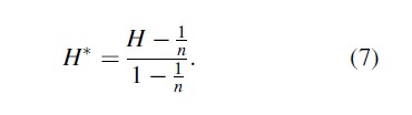
As with the previous two measures of specialization, the Diversity Index is a general measure of specialization and does not provide information regarding what type of crime classification specialization occurs in a particular subregion.

The following measure of specialization has not been given a name in the economics literature, so it will simply be referred to as the Specialization Index in this discussion. The Specialization Index is calculated as follows:

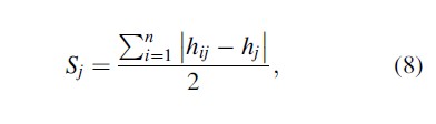
where h_ij is the share of crime j at subregion i and h_j is the share of crime j in the study area as a whole. The Specialization Index ranges from zero to unity with unity representing total specialization. The Specialization Index does not provide information regarding which type of crime classification specialization occurs in a particular subregion.

The last measure of specialization considered here is the Entropy Index – this index has been used in the public health literature to measure mixed land use (Frank et al. 2004). The Entropy Index for area j is calculated as follows:

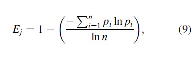
where p_i represents the share of crime classification i and n is the total number of crime classifications. The Entropy Index ranges from zero (evenly distributed crime classifications) to unity (perfect specialization). As with all the alternative measures of specialization, the Entropy Index does not provide information regarding what type of crime classification specialization occurs in a particular subregion. Also, as with the Theil Index, the Entropy Index has difficulties dealing with zero values for p_i because ln(0) is undefined. However, in this case ln(0) may be set to zero without loss of meaningful interpretations.

There are, of course, many other measures of specialization, primarily stemming from the economics, geography, and regional sciences literatures. Though they vary in the details, they generally convey the same type of information as those shown above. The primary difference between the measures shown above and other measures of specialization found in the literature is the complexity of the calculation. However, at this stage of introducing alternative measures of specialization that may be used in the context of places, the more straightforward measures were chosen to show their utility.

Mapping The Alternative Measures Of Specialization

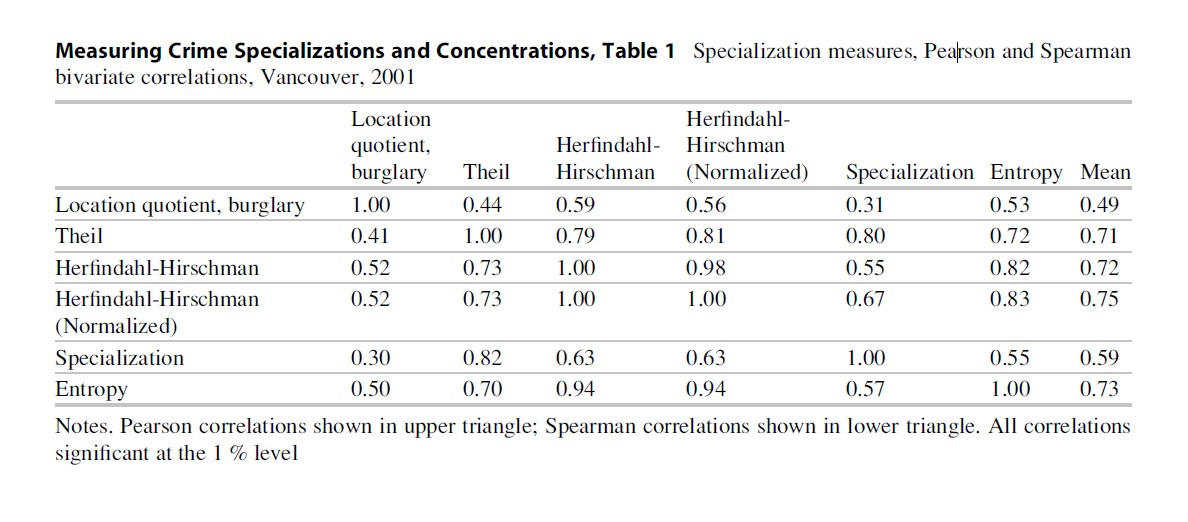
Before the discussion turns to the maps of the alternative measures of specialization, the similarity between the various alternative measures (and the location quotient for burglary) is of interest. The bivariate correlations (Pearson and Spearman) are shown in Table 1: Pearson correlations are shown in the upper right triangle of the table, whereas Spearman correlations are shown in the lower right triangle of the table. Though the location quotient for burglary is not highly related to the other measures of specialization (the correlations are positive and statistically significant), the alternative measures of specialization are, generally speaking, highly related with each other. Such relationships are not particularly surprising because the location quotient for bur glary only considers burglary and the alternative measures of specialization are all quantifying the general nature of specialization, not being concerned with any particular crime. In fact, most of the (Pearson) correlations between the alternative measures of specialization are approximately 0.80, indicating that there is significant interchangeability among these alternative measures of specialization. The maps of these alternative measures indicate a similar conclusion.

Of all the alternative measures of specialization discussed above, only four are mapped for subsequent discussion: Theil Index (Fig. 2a), HerfindahlHirschman (Normalized) Index (Fig. 2b), Specialization Index (Fig. 2c), and Entropy Index (Fig. 2d) – the normalized location quotient is not mapped because the results are so similar to the location quotient shown in Fig. 1b, and the Herfindahl-Hirschman Index is not mapped because of its similarity to the HerfindahlHirschman (Normalized) Index. Because there are no classifications for these four alternative measures, unlike the location quotient, they are shown using natural breaks and five groups.

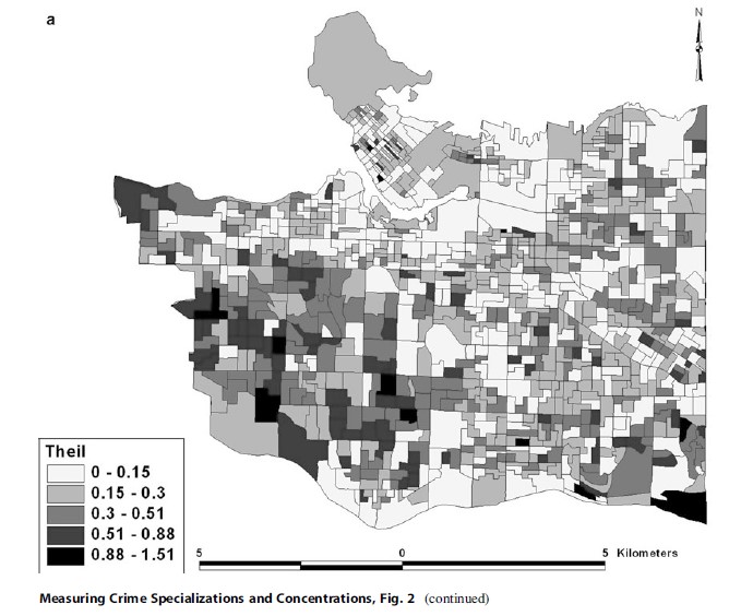
Immediately obvious with the Theil Index (Fig. 2a) is that the spatial pattern is similar to that of the location quotient for burglary (Fig. 1b). Though the spatial pattern is not as strong as with the location quotient, crime appears to specialize within the western side of Vancouver. This pattern is the opposite of expected when considering crime concentration because the west side of Vancouver is the wealthier section of the city – it contains some of the wealthiest neighborhoods. The DAs that have the greatest concentration is a smaller area than the similar classification for the location quotient for burglary, but is present nonetheless. The difficulty with this mapped output, as mentioned above, is that the Theil Index is a general measure of specialization and the research is forced to ask: specializes in what?

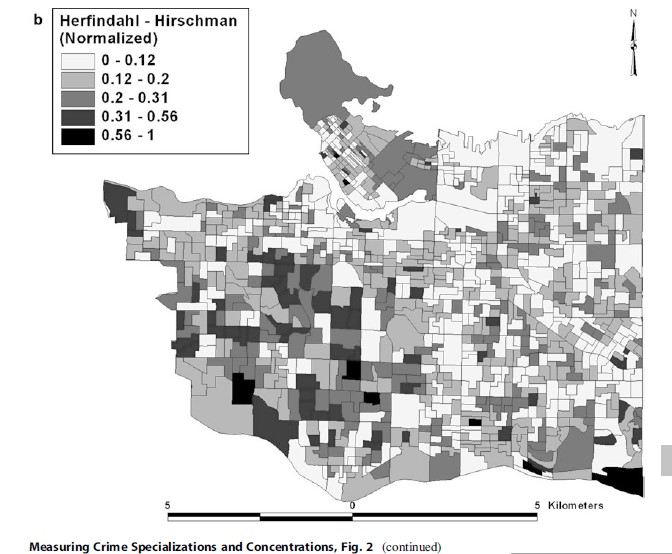
The Herfindahl-Hirschman (Normalized) Index (Fig. 2b) shows a similar pattern to that of the Theil Index: crime concentration in the western port of Vancouver, but not nearly as much as shown using the location quotient for burglary. Also noteworthy are the legend categories for the Herfindahl-Hirschman (Normalized) Index. Inspection of the legend and the mapped output reveals that there are not many DAs that have index values greater than 0.50. This is not problematic but shows that the Herfindahl-Hirschman (Normalized) Index is a more conservative measure of specialization than the Theil Index.

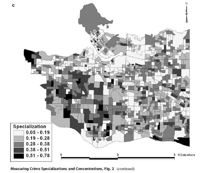
The Specialization Index (Fig. 2c) has the same general pattern as shown in Figs. 2a and 2b but is a blend of these two specialization indices: the mapped output for Specialization Index is more similar to the Theil Index, but the legend categories are more similar to the Herfindahl-Hirschman (Normalized) Index. The primary difference that emerges with the Specialization Index is that there are more DAs that exhibit specialization than in the previous two alternative measures of specialization.

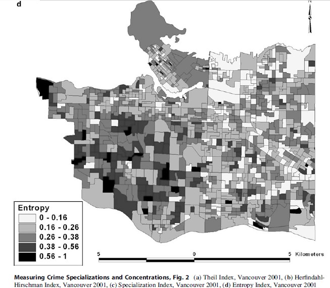
Lastly, the Entropy Index (Fig. 2d) again exhibits a similar spatial pattern to the previous alternative measures of specialization. However, the number of DAs that show a high degree of specialization using the Entropy Index is rather low. Overall, and not surprising given the high magnitude correlations between the different measures of specialization (Table 1), the spatial patterns of the different alternative measures of specialization are quite similar.

Future Directions For Crime Specialization

This research paper has discussed the need to separately consider crime concentration and crime specialization, presented the location quotient and reviewed the criminological literature that has employed the location quotient, and presented and mapped some alternative measures of specialization. It has also opened the debate on which method might prove the most useful in measuring crime specialization. Though the different measures of specialization vary in their calculations, the output of these different measures of specialization is remarkably similar. This indicates that the choice of which measure of specialization the research decides to use has little impact on the overall spatial pattern – all of the alternative measures of specialization are general measures in that they do not show which crime classification an area is specializing in.

Because of this, unless there are very few zero values for crime in an analysis, the Theil Index and the Entropy Index are not ideal in the context of crime in smaller areal units of analysis (microplaces). This leaves the Herfindahl-Hirschman (Diversity) Index and the Specialization Index. Because of its current use in the criminological literature and its ease of calculation, the Herfindahl-Hirschman (Diversity) Index is probably the best of all the alternatives.

Again, the researcher is still left to ask: this place specializes in which crime? It is recommended that an initial measure of specialization, generally speaking, be calculated to investigate whether or not any specialization exists. If specialization does occur, then the time may be taken to calculate the various location quotients for each crime classification under analysis. In the case of Vancouver, only burglary specializes in the spatial patterns evident in Fig. 2a-d. As such, the alternative measures of specialization all indicate that specialization does indeed occur in Vancouver and the location quotient can then be used to identify what type of specialization is taking place. This information may then be used to identify the opportunity surface relative to each crime classification to understand the particulars of crime specialization.

With the respective opportunity surfaces identified, an obvious extension is to find what drives the specialization of different crime classifications. In other words, why is crime specialization particularly conspicuous in certain places? There are a number of data sources that may prove instructive for this endeavor. The census is an obvious data set that is available to most researchers. However, because of the time lag between census years (as long as 10 years), these data may not be the most reliable. Another data source that has proven useful in identifying crime generators and crime attractors is land use data (Kinney et al. 2008); Kinney et al. (2008) found that crime generators and crime attractors are best identified using highly specific land use classifications. It is expected to be similar for crime specialization.

Lastly, with information regarding the presence of crime specialization, the location of crime specialization, and why it is present in certain places, this may be used to inform policy decisions. Specifically, such information may be of interest to police in order to address specific crime issues. For example, the police may not only be interested in burglary in the places where it is most frequent (based on counts) but also in the places where it is the most problematic even if its incidence level is not particularly high. Similarly, this information may be of use for crime prevention initiatives, more generally, not just policing.

Bibliography:

1. Andresen MA (2006) Crime measures and the spatial analysis of criminal activity. Br J Criminol 46:258–285
2. Andresen MA (2007) Location quotients, ambient populations, and the spatial analysis of crime in Vancouver, Canada. Environ Plann A 39:2423–2444
3. Andresen MA (2009) Crime specialization across the Canadian provinces. Can J Criminol Crim Justice 51:31–53
4. Andresen MA, Malleson N (2011) Testing the stability of crime patterns: implications for theory and policy. J Res Crime Delinq 48:58–82
5. Balassa B (1965) Trade liberalisation and “revealed” comparative advantage. Manchester Sch Econ Soc Stud 33:99–123
6. Block S, Clarke RV, Maxfield MG, Petrossian G (2012) Estimating the number of U.S. vehicles stolen for export using crime location quotients. In: Andresen MA, Kinney JB (eds) Patterns, prevention, and geometry of crime. Routledge, New York, pp 54–68
7. Brantingham PL, Brantingham PJ (1981) Notes of the geometry of crime. In: Brantingham PJ, Brantingham PL (eds) Environmental criminology. Waveland Press, Prospect Heights, pp 27–54
8. Brantingham PL, Brantingham PJ (1993) Location quotients and crime hot spots in the city. In: Block CR, Dabdoub M (eds) Workshop on crime analysis through computer mapping, proceedings. Criminal Justice Information Authority, Chicago. pp 175–197
9. Brantingham PL, Brantingham PJ (1995) Location quotients and crime hot spots in the city. In: Block CR, Dabdoub M, Fregly S (eds) Crime analysis through computer mapping. Police Executive Research Forum, Washington, DC, pp 129–149
10. Brantingham PL, Brantingham PJ (1998) Mapping crime for analytic purposes: location quotients, counts and rates. In: Weisburd D, McEwen T (eds) Crime mapping and crime prevention. Criminal Justice Press, Monsey, pp 263–288
11. Bulwer HL (1836) France, social, literary, political, volume I, book I: crime. Richard Bentley, London
12. Clarke RVG, Cornish DB (1985) Modeling offenders’ decisions: a framework for research and policy. Crime Justice Annu Rev Res 6:147–185
13. Cohen LE, Felson M (1979) Social change and crime rate trends: a routine activity approach. Am Sociol Rev 44:588–608
14. De Benedictis L, Gallegati M, Tamberi M (2009) Overall trade specialization and economic development: countries diversify. Rev World Econ 145: 37–55
15. Eck JE, Weisburd D (eds) (1995) Crime prevention studies, volume 4, crime and place. Criminal Justice Press, Monsey
16. Frank LD, Andresen MA, Schmid TL (2004) Obesity relationships with community design, physical activity, and time spent in cars. Am J Prev Med 27:87–96
17. Herfindahl OC (1950) Concentration in the U.S. steel industry. Unpublished doctoral dissertation, Columbia University
18. Hirschman AO (1945) National power and the structure of foreign trade. University of California Press, Berkeley
19. Johnson SD, Summers L, Pease K (2009) Offender as forager? A direct test of the boost account of victimisation. J Quant Criminol 25:181–200
20. Kinney JB, Brantingham PL, Wuschke K, Kirk MG, Brantingham PJ (2008) Crime attractors, generators and detractors: land use and urban crime opportunities. Built Environ 34:62–74
21. McCord ES, Ratcliffe JH (2007) A micro-spatial analysis of the demographic and criminogenic environment of drug markets in Philadelphia. Aust N Z J Criminol 40:43–63
22. Miller MM, Gibson LJ, Wright NG (1991) Location quotient: a basic tool for economic development studies. Econ Dev Rev 9:65–68
23. Quetelet LAJ (1842) A treatise on man and the development of his faculties. W and R. Chambers, Edinburgh
24. Ratcliffe JH (2001) On the accuracy of TIGER type geocoded address data in relation to cadastral and census areal units. Int J Geogr Inf Sci 15:473–485
25. Ratcliffe JH (2004) Geocoding crime and a first estimate of a minimum acceptable hit rate. Int J Geogr Inf Sci 18:61–72
26. Ratcliffe JH, Rengert GF (2008) Near repeat patterns in Philadelphia shootings. Secur J 21:58–76
27. Rengert GF (1996) The geography of illegal drugs. Westview Press, Boulder
28. Sherman LW, Gartin PR, Buerger ME (1989) Hot spots of predatory crime: routine activities and the criminology of place. Criminology 27:27–56
29. Theil H (1967) Economics and information theory. Rand McNally, Chicago
30. Weisburd D, Groff ER, Yang S (2012) The criminology of place: street segments and our understanding of the crime problem. Oxford University Press, New York

See also:

• How to Write a Research Paper
• Research Paper Topics
• Research Paper Examples

Free research papers are not written to satisfy your specific instructions. You can use our professional writing services to buy a custom research paper on any topic and get your high quality paper at affordable price.