Spatial Models and Network Analysis Research Paper

This sample Spatial Models and Network Analysis Research Paper is published for educational and informational purposes only. If you need help writing your assignment, please use our research paper writing service and buy a paper on any topic at affordable price. Also check our tips on how to write a research paper, see the lists of criminal justice research paper topics, and browse research paper examples.

Several issues in criminology have led to the widespread use of spatial econometric statistical models. This research paper outlines the principles and concepts behind the use of spatial models in criminology, including a description of the most commonly used models in spatial criminology. Next is a discussion of a critical but often overlooked element of spatial model specification, the construction of the spatial weights matrix, which should be theory dependent. The paper concludes with a discussion of the limitations of distance-or proximity-based approaches to constructing the spatial weights matrix, including the use of social network analysis to overcome these limitations.

Foundations Of Spatial Modeling In Criminology

The recognition of geography as a factor in the explanation of a multitude of social phenomena has been an increasingly notable component of quantitative criminology. Research concerned with basic and applied questions pertaining to crime, criminal justice, and policy now typically incorporate geographic or spatial elements into analyses that utilize quantitative methodologies. An important reason for the adoption of spatial perspectives for quantitative criminology has been a growing recognition of the importance of context to human action. Incorporating context into quantitative models of human behavior is an ongoing focus of the subfield of spatial criminology.

The analysis of spatial phenomena in criminology has been made possible in recent years by the ongoing development of statistical techniques that attempt to deal with some of the unique problems of spatial data, especially spatial dependence. Dependence, or the tendency of characteristics of a given location to correlate with those of nearby locations, is a foundational issue in quantitative geographical analysis (e.g., Anselin 1988). When present in spatially organized data, spatial dependence can result in the spatial autocorrelation of regression residuals, which simply means that the values of variables sampled at nearby locations are not independent from each other (such values may be either positively or negatively correlated). The presence of spatial autocorrelation may lead to biased and inconsistent regression model parameter estimates and increase the risk of a type I error (falsely rejecting the null hypothesis). Accordingly, a critical step in statistical model specification when using spatial data is to assess the presence of spatial autocorrelation.

The statistical models developed to deal with spatial dependence, commonly called spatial econometric models, are now increasingly of interest to researchers from diverse disciplines investigating a wide range of issues, including crime and criminal justice. Many criminologists utilizing quantitative techniques now view spatial econometric regression models as an improvement non-spatial techniques as a result of the growing recognition that dependencies in the spatial structure of research data limit the reliability of inferences from conventional regression models (Anselin 1988). While there are now a variety of methods to address spatially auto correlated data in regression models, the standard workhorse in spatial regression is what are commonly referred to as simultaneous autoregressive (SAR) models.

SAR models can take three different basic forms (see Anselin 1988, 2002). The first SAR model assumes that the autoregressive process occurs only in the dependent, or response, variable. This is called the “spatial lag” model, and it introduces an additional covariate to the standard terms for the independent or predictor variables and the errors used in an ordinary least squares (OLS) regression (the additional variable is referred to as a “spatial lag” variable which is a weighted average of values for the dependent variable in areas defined as “neighbors”). Drawing on the form of the familiar OLS regression model and following Anselin (1988), the spatial lag model may be presented as

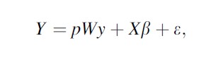
Spatial Models and Network Analysis Research Paper

where Y is the dependent variable of interest, r is the auto regression parameter, W is the spatial weights matrix, X is the independent variable, and e is the error term.

The second SAR model assumes that the autoregressive process occurs only in the error term. In this case, the usual OLS regression model is complemented by representing the spatial structure in the spatially dependent error term. The error model may be presented as

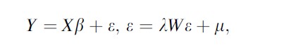
Spatial Models and Network Analysis Research Paper

where λ is the auto regression parameter and e is the error term composed of a spatially auto correlated component (W ε) and a stochastic component (μ) with the rest as in the spatial lag model.

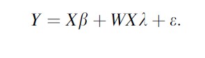
The third SAR model can contain both a spatial lag term for the response variable and a spatial error term, but is not commonly used. Other SAR model possibilities include lagging predictor variables instead of response variables. In this case, another term must also appear in the model for the auto regression parameters (y) of the spatially lagged predictors (WX). This model takes the form

Spatial Models and Network Analysis Research Paper

Combining the response lag and predictor lag terms in a single model is also possible (sometimes referred to as a “mixed” model).

As Anselin (1988) observes, spatial dependence has much to do with notions of relative location between units in potentially different kinds of space, such as a conceptual social space. Accordingly, SAR models share a number of common features with network autocorrelation models. Substantively, spatial and network approaches have been used to explore similar questions pertaining to influence and contagion effects, albeit among different units of observations (see Marsden and Friedkin 1993 for examples). In such cases proximity or connectedness is assumed to facilitate the direct flow of information or influence across units. Individuals or organizations are also more likely to be influenced by the actions, behaviors, or beliefs of others that are proximate on different dimensions, including geographical and social space.

The Spatial Weights Matrix (W)

Spatial econometric regression models demand a careful consideration of both the theoretical and empirical spatial structure of the data in question (e.g., Florax and Rey 1995). However, the advent of new spatial econometric software packages has lowered the traditional technical barriers to the use of these techniques while simultaneously making it easy for users to choose among a few predefined spatial structures. New users may therefore be unfamiliar with the importance of the formal spatial structure to analytic outcomes and less likely to carefully consider their choice (Leenders 2002). The small literature new users may draw upon to understand this issue remains quite technical in nature, even when proclaiming the opposite intent (e.g., Griffith 1996). Taken as a whole, this state of affairs is less than ideal and unlikely to encourage careful thinking about space. However, the need to formalize the empirical spatial structure of the data for modeling is also an opportunity to reflect on the theoretical interaction of the geography and social processes being studied. In this manner, spatial analyses of human behavior and outcomes are at the core of an emerging “spatially integrated social science” identified by Goodchild et al. (2000), and an opening for the investigation of how human behavior and space is mutually constituted.

As typically argued in many geographic literatures and increasingly in quantitative criminology, spatial perspectives are important for both theoretical and practical reasons. Theoretically, spatial perspectives are of interest because of the long-standing interest in the social production of space in geography. Following Lefebvre’s (1991) understanding of space as both social process and social product, the spatial structures of a given phenomenon are commonly investigated as underlying cause, constructed outcome, or both. For example, the perception of rivalries over territorial control between a set of gangs and the actual construction of bounded turf are simultaneously a social and a geographic phenomenon. The competitions are inseparable from the geography and vice versa. Hence modeling a social process such as gang rivalry requires a consideration of the modeling the social construction of space (Radil et al. 2010).

On the other hand, consideration of geography is a practical methodological matter. Data with a geographical component has important implications for statistical analyses; if processes that are affected by the underlying spatial structure in a study area are not accounted for, inferences will be inaccurate and estimates of the effects of independent variables may be biased (Anselin 1988). Perhaps the most important reason for the interest in quantitative spatial methods is the most straightforward: nearly all social science data is spatially organized, and ignoring this structural element is increasingly seen as untenable. To accommodate these issues, statistical models have been developed that attempt to deal with issues of spatial dependence. Conventionally, this is done through either introducing an additional covariate (the “spatial lag” variable discussed in the previous section) or by specifying a spatial stochastic process for the error term.

These models, now seen as both viable and important for social science research, have been discussed and exemplified in depth (see Anselin 2002 for an overview), but an essential element of these models remains largely ignored in the literature, despite the major theoretical and methodological implications. Both the lag and error models attempt to estimate regression parameters in the presence of presumably interdependent variables (Anselin 1988; Leenders 2002). This estimation process requires the analyst to define the form and limits of the interdependence and formalize the influence one location has on another. In practice, this is accomplished by identifying the connectivity between the units of the study area through a n× n matrix. The matrix is usually described in the literature as a “spatial weight” or “spatial connectivity” matrix and referred to in the preceding SAR models as “W.” This W, or matrix of locations, formalizes

a priori assumptions about potential interactions between different locations, defining some locations as influential upon a given location and ruling others out. A simpler way of describing this is that W identifies, in some cases, who is a neighbor and who is not or with whom an actor interacts. However, the construction of W is more than just an empirical choice about neighbors. It is a theoretical decision regarding the spatiality of the social processes being discussed and one that has implications for the statistical estimates generated.

As W is supposed to represent a formal model of connections between geographic locations, how one translates theories about influence and its mechanisms across space into a formal mathematical construct is an important step. Put another way, at its core, W is really a theoretical geography of interaction. However, as a practical matter, the spatial analytic geography literature focuses on modeling interaction through a distance-based logic that typically takes one of two forms: contiguity or distance (Cliff and Ord 1981; Griffith 1996). Both of these spatial themes have been mobilized for constructing Ws for various kinds of measures of spatial autocorrelation dating back to Cliff and Ord’s seminal work (1981). Contiguity, or the physical connections between locations, is emphasized in issues that focus on areal spaces, especially ecological studies that use aggregated data and attempt to evaluate the relationships between neighborhood composition and crime outcomes. Distance between locations of interest also remains an important concept for criminology, in particular for journey-to-crime research.

Theorizing W With Social Network Analysis

Whether contiguity-or distance-based, the geography of influence is typically imagined and implemented in SAR models as a kind of gradient that uniformly diminishes with increasing distance, also known as the concept of distance decay (see Stephenson 1980). Classic examples of distance-decay thinking in social science are Boulding’s (1962) “loss of strength gradient” which argued that military power has a direct inverse relationship with distance and Tobler’s (1970) so-called “first law” of geography which states that everything is related to everything else, but near things are more related than are far things.

At a basic level, distance decay is the foundational concept behind the implementation of W in most spatial economic models, and the development and dissemination of spatial analytic software allow users to easily create Ws from spatially organized data using the classic spatial forms of areal contiguity or point-to-point distance. While such software often guides researchers through the practical steps needed to create a matrix of spatial interaction or influence grounded in distance decay, there is no drop-down menu to offer guidance as to how best to capture the specific geography, or spatiality, of the social processes being analyzed. For any given research topic, are immediately contiguous areal neighbors enough, or should more distant neighbors also be included? If distance matters, at what distance does influence begin to diminish? Does influence diminish over distance in the same way for all social actors or behaviors? More to the point, why and in what way does distance “matter” in the operation of the social process under investigation? Addressing these sorts of questions remains the key challenges for a theoretically informed spatial analysis in criminology.

Somewhat surprisingly, theoretical discussions about the nature of W and practical discussions of how different specification choices may affect regression results have also been underemphasized in most spatial analytic literature. Despite these noteworthy efforts, Leenders (2002: 44) is correct in his assessment that “the effort devoted by researchers to the appropriate choice of W pales in comparison to the efforts devoted to the development of statistical and mathematical procedures.” The net effect of this lack of attention is that theoretical conceptions about the role space plays in producing empirical patterns in a given dataset are often afterthoughts and little effort is given to understanding how sensitive model results may be to different specifications of W. Hence, the vision of a “spatially integrated social science” (Goodchild et al. 2000) remains unfulfilled, because when space is included in the analysis of social processes, it is often added in a default form without consideration of the geographic expression of the processes in question.

Criminologists have begun to explore such questions, often turning explicitly to the concept of social networks and the associated field of social network analysis. For example, social networks within neighborhoods are often implicated as being important mechanisms in the production and maintenance of safe, low-crime neighborhoods (e.g., Sampson et al. 1997). Such approaches argue that individual-level social bonds among local residents facilitate the formation of informal social control and the creation of shared goals and trust that regulate and censure local activities. A general acceptance of the importance of networks of local social relationships for understanding rates and patterns of neighborhood crime has prompted researchers to look into the kinds of social networks operating in communities in an effort to gather information regarding social ties among local residents as well as peer associations with delinquent others.

Beyond examining the degree to which individual-level ties influence crime patterns within a community, researchers are also beginning to explore the importance of institutional or organizational ties that can bridge communities. Sampson (2004: 158) argues for reconceptualizing neighborhoods “as nodes in a larger network of spatial relations” in order to account for the various ties that can link residents across space. Although Sampson (2004) does not specifically suggest what kinds of local institutions or organizations one should consider as important to explaining crime, in general terms he refutes the notion that neighborhoods are analytically independent and argues that ecological models of crime need to consider the different ways in which the observable outcomes in one neighborhood are partly the product of social actions and activities that can stretch beyond local communities (Morenoff et al. 2001; Sampson 2004).

Drawing on such arguments about the importance of both localized and no localized social networks, an emerging framework in quantitative criminology argues for a “deductive approach” to incorporating space built on the understanding that social networks are inherently geographic, existing both within and across localities and connecting communities separated by distance (e.g., Radil et al. 2010; Tita and Radil 2010). This analytic framework allows influence to take place not just between geographically proximate neighbors (as with conventional distance-decay-based spatial regression models) but also between locations that are connected directly by social networks. By carefully considering and allowing for processes that extend beyond (or perhaps preclude) spatially adjacent areas, one can ensure that the spatial weights matrix adequately captures the realities of the mechanisms of influence. Just as Morenoff (2003: 997) argues that spatial analysis “expands the neighborhood-effects paradigm by considering not only the local neighborhood but also the wider spatial context within which that neighborhood is embedded,” a careful consideration of the spatial dimensions of social influence is under way as part of an attempt to facilitate the inclusion of the “wider social context of neighborhoods” into quantitative models of crime.

An early example of this emerging framework was found in the work of Mears and Bhati (2006), which links adjacent as well as nonadjacent areas to one another if the residents are economically and demographically similar by constructing W based on “similarity” that links socially similar areas together regardless of spatial proximity. Most recently, this framework has been advanced by research into the importance of both social and spatial linkages among gangs embedded within various types of local networks (Tita and Greenbaum 2009; Radil et al. 2010; Tita and Radil 2010). Rather than inferring connections through social similarity, the framework first demonstrated by Tita and Greenbaum (2009) accounts for influence by simultaneously considering linkages through geographic proximity between neighborhoods as well as through specific social ties that connect places. This approach carefully identifies direct social connections between neighborhoods based on rivalries between urban street gangs that are not geographically proximate, while also preserving the underlying spatial structure of the entire study area. Tita and Radil (2010) examined the utility of such an approach by comparing spatial regression model outcomes of gang violence using three differently constructed Ws based on geographic adjacency, social connectivity, and a blend of both. Tita and Radil (2010) argued that violence committed by, and against, gang members in a socially and geographically distinct area of Los Angeles is largely a function of a social process that spans the local geography in such a way that violence in noncontiguous areas impacts levels of violence in a focal neighborhood and that blended W that incorporated both distance-based spatial effects and connections formed by specific social relations across neighborhoods offered the most meaningful results to the explanation of gang violence, both theoretically and statistically.

These studies reflect a growing interest and recognition in quantitative criminology of the need to not simply incorporate space and spatial effects in the study of crime but to do so in a way that moves beyond the uncritical notions of uniform distance decay that underpin SAR models. Specifications of the spatial weights matrix, or W, that rely solely on spatial contiguity or distance to define the spatial reach of the various social processes posited to be responsible for clustering force researchers to assume that all such processes decay rapidly and uniformly over geographic distance and therefore matter only among spatially adjacent neighbors. Furthermore, even when multiple social processes are considered, the conventional modeling approach has been to specify a single W rather than specify different kinds of connections between places for different social processes. In addition to making it impossible to parse the impact of one process from that of another, this is an a theoretical approach to understanding why and how space matters (Leenders 2002). By carefully considering the socio-spatial dimensions of the criminal phenomena of interest and of the actors behind them, the work of Mears and Bhati (2006) and (Tita and Radil 2010) demonstrate new possibilities by creating Ws that explicitly capture the social and geographic dimensions of spatial influence through incorporating social networks. Further, such approaches allow theories of spatial influence to guide the construction of W, a meaningful advance given Leenders’ (2002) concern with the lack of careful consideration of the underlying social processes of influence exhibited by researchers in their construction of weights matrices.

This is not to say that all the challenges of incorporating space into studies of crime have been met. For example, the developing arguments about the importance of microscale units of analysis in criminology (Hipp 2007) complicate the need to model interaction as the likelihood for spillover or other unmeasurable spatial effects increases as the areal scale of the unit of analysis decreases. Additional challenges include the need to incorporate dynamism and change over time in social networks and space and the need to consider overlapping networks (Ettlinger 2003) or multiple spatialities (Leitner et al. 2008) when theorizing the interactions between people and space. Nonetheless, the value of theoretically grounded notions of the geographic complexities of the mechanisms of influence in terms of positing various theories and mechanisms responsible for observable patterns of crime cannot be overstated. The current efforts underway in quantitative criminology have demonstrated the value of employing such an approach which should encourage future research into how social networks are involved in the social production of space and how the methods of social network analysis may be further utilized to understand if and how the structure of social networks have implications for material geographies of crime.

Bibliography:

Anselin L (1988) Spatial econometrics: methods and models. Kluwer, Boston
Anselin L (1998) Exploratory spatial data analysis in a geocomputational environment. In: Longley P, Brooks S, McDonnell R, Macmillan B (eds) Geocomputation, a primer. Wiley, New York
Anselin L (2002) Under the hood: issues in the specification and interpretation of spatial regression models. Agric Econ 27(3):247–267
Anselin L, Florax R, Rey S (2004) Advances in spatial econometrics: methodology, tools and applications. Springer, Berlin
Boulding K (1962) Conflict and defense. Harper, New York
Cliff A, Ord J (1981) Spatial processes, models, and applications. Pion, London
Ettlinger N (2003) Cultural economic geography and a relational and microspace approach to trusts, rationalities, networks, and change in collaborative workplaces. J Econ Geogr 3(2):145–171
Florax R, Rey S (1995) The impacts of misspecified spatial interaction in linear regression models. In: Anselin L, Florax R (eds) New directions in spatial econometrics. Springer, Berlin, pp 111–135
Goodchild M, Anselin L, Appelbaum R, Harthorn B (2000) Toward spatially integrated social science. Int Reg Sci Rev 23:139–159
Griffith D (1996) Some guidelines for specifying the geographic weights matrix contained in the spatial statistical models. In: Arlinghaus S (ed) Practical handbook of spatial statistics. CRC Press, Boca Raton, pp 65–82
Hipp J (2007) Block, tract, and levels of aggregation: neighborhood structure and crime and disorder as a case in point. Am Sociol Rev 72:659–680
Leenders R (2002) Modeling social influence through network autocorrelation: constructing the weight matrix. Soc Netw 24:21–47
Lefebvre H (1991) The production of space (trans: Nicholson-Smith D). Blackwell, Oxford/Basil
Leitner H, Sheppard E, Sziarto K (2008) The spatialities of contentious politics. Trans Inst Br Geogr 33(2):157–172
Marsden P, Friedkin N (1993) Network studies of social influence. Soc Methods Res 22:125–149
Mears D, Bhati A (2006) No community is an island: the effects of resource deprivation on urban violence in spatially and socially proximate communities. Criminology 44(3):509–548
Morenoff J (2003) Neighborhood mechanisms and the spatial dynamics of birth weight. Am J Sociol 108:976–1017
Morenoff J, Sampson R, Raudenbush S (2001) Neighborhood inequality, collective efficacy, and the spatial dynamics of urban violence. Criminology 39:517–560
Radil S, Flint C, Tita G (2010) Spatializing social networks: using social network analysis to investigate geographies of gang rivalry, territoriality, and violence in Los Angeles. Ann Assoc Am Geogr 100(2):307–326
Sampson R (2004) Networks and neighborhoods: the implications of connectivity for thinking about crime in the modern city. In: McCarthy H, Miller P, Skidmore P (eds) Network logic: who governs in an interconnected world? Demos, London, pp 157–166
Sampson R, Raudenbush S, Earls F (1997) Neighborhoods and violent crime: a multilevel study of collective efficacy. Science 277:918–924
Stephenson L (1980) Central graphic analysis of crime. In: Georges-Abeyie D, Harries K (eds) Crime: a spatial perspective. Columbia University Press, New York, pp 146–155
Tita G, Greenbaum R (2009) Crime, neighborhoods and units of analysis: putting space in its place. In: Weisburd D, Bernasco W, Bruinsma G (eds) Putting crime in its place: units of analysis in spatial crime research. Springer, New York, pp 145–170
Tita G, Greenbaum R (2011) Spatializing the social networks of gangs to explore patterns of violence. J Quant Criminol 27(4):521–545
Tita G, Radil S (2010) Making space for theory: the challenges of theorizing space and place for spatial analysis in criminology. J Quant Criminol 26(4):467–479
Tobler W (1970) A computer movie simulating urban growth in the Detroit region. Econ Geogr 462:234–240
Weisburd D, Bernasco W, Bruinsma G (eds) (2009) Putting crime in its place: units of analysis in spatial crime research. Springer, New York