Understanding Victimization Frequency Research Paper

This sample Understanding Victimization Frequency Research Paper is published for educational and informational purposes only. If you need help writing your assignment, please use our research paper writing service and buy a paper on any topic at affordable price. Also check our tips on how to write a research paper, see the lists of criminal justice research paper topics, and browse research paper examples.

In the past two decades, the central place of repeat and multiple crime incidents against the same victims in boosting crime rates, predicting vulnerability to victimization and, with that knowledge, assisting crime prevention, has been recognized. This research paper overviews the accumulated evidence on measuring and predicting victimization frequency and hints at possible crime prevention implications. It concludes with a list for future improvements in measuring and thus understanding repeat victimization.

Context

The field of criminology has traditionally focused on the offenders, the origins of offending behavior, and how to contain or ultimately eliminate it. The Chicago School of the inter-world war period broke away from that tradition by examining the societal (demographic, social, and economic) conditions that were associated with crime concentration. In doing so, researchers, such as Shaw and McKay (1942), introduced context to the study of crime and examined the conditions that enabled offending propensities to be formed and acted out. Since then, considerable research has been conducted in this vein and valuable lessons have been learned while Chicago still yields some groundbreaking analyses of the contextual behavioral parameters of crime concentration (Sampson 2006)!

The development of criminology via the study of offending in relation to area crime concentration has been encouraged and facilitated by the type of information that has been available to researchers and practitioners alike. Police records and data from other criminal justice agencies have existed roughly since the formation of these institutions (readers are invited to explore the rich archive held by the Galleries of Justice located in the old Sheriff of Nottingham mansion, court, prison, and “serious” offenders’ execution site of the writer’s home city should they visit it). Recorded crime data however hold only basic, if any, information on the victims of crime, such as name, sex, and age. As police alongside other state/public institutions’ accountability came into question, it became clear that recorded crime gives a partial picture of how much crime is committed. Population-based criminal victimization surveys were thus launched in the 1970s as a means to estimate the “dark” figure of crime and implicitly or explicitly evaluate the quality and efficiency of the police service. Victims of crime, who at that time were conveniently distinguished from offenders, came, therefore, to the forefront of criminological enquiry to offer information about the criminal incidents they have experienced, the circumstances of their occurrence, and any consequences to those involved.

The National Crime Survey was launched in 1973 in the USA as a tool to “measure” crime in society. After two decades, it was revamped as the National Crime Victims Survey (NCVS) with improved information about victim and crime situational characteristics. In 1981, the British Crime Survey (BCS) was launched in the UK to offer data to supplement that on recorded crime (with regular sweeps in England and Wales) and provide appropriate measurements for testing victimization theory and crime-related national policy initiatives. National crime surveys have also been introduced in Canada, Australia/ New Zealand, and a number of European countries. In 1989, the first regular comparative survey was launched, the International Victimization Survey, which followed the same sampling design and administered the same questionnaire cross-nationally until recently (2005). Since 2000, it has been known as the International Criminal Victimization Survey (ICVS). For many countries and some parts of the world, the ICVS is the only crime survey data held. The above are the main data sources upon which this research paper draws.

The pioneering victimization research that originated from the forerunner to the NCVS and resulted in the well-known lifestyle theory examined the association between the likelihood of experiencing crime and each socioeconomic attribute at hand (Hindelang et al. 1978). For instance, whether victims belonged disproportionally to specific population subgroups was assessed in an effort to identify “victim profiles” in a similar manner to that by which offender characteristics had been and continue to be drawn. The victimization theories of lifestyle and routine activities are well documented in the literature and textbooks (Felson 2002). The developments in statistical modeling research of the last two decades have shown that lifestyle and routine activity effects alone do not predict victimization and that context, that is, the social disorganization parameters put forward by Shaw and McKay (1942), is equally important (for instance, Kennedy and Forde 1990; Osborn and Tseloni 1998). Finally, the appearance in the new millennium of studies based on hierarchical modeling established that individual characteristics and lifestyles are not only additional factors to but also conditioned by context (Rountree et al. 1994; Tseloni 2000) as well as victimization history (Tseloni and Pease 2004). Therefore, a micro-and macro-level victimization theory seems to be emerging that recognizes the context-specific importance of socioeconomic attributes, routine activities, and previous crime experiences. This work will not revisit the original theories but dwell on the established evidence that the world, victimization not excepted, is a multi-dimensional place.

The Pervasiveness Of Victimization: Definitional Issues

This part focuses on the different ways in which victimization and victims can be defined. This is central in understanding, predicting, and thus preventing criminal victimization.

The likelihood of becoming victim of crime, also known as victimization risk or prevalence, gives the probability that a crime target experiences at least one crime incident during a specific period. The population of eligible crime targets varies according to the crime type in question. For instance, personal crimes may affect any individual in a society, property crimes are against households, or car theft refers to the number of car-owning households. The specific period that offers a snapshot of crime problems in a society depends on the sampling design and the nature of the employed survey. It can be, for instance, the quarter, the calendar year (January to December), the financial year (April to March), or a lifetime.

Victimization risk has been widely used and still appears as the main variable of interest in empirical research. However, it confounds a wide spectrum of victim experiences, from unlucky chance encounters to dangerous daily lives. Therefore, examining the all-encompassing probability of being victimized one or more times does not tell much about the mechanisms of criminal victimization and, therefore, how to prevent it. Indeed, each victim type from the typology set out below represents quite different crime experiences affecting the perceived seriousness of that experience (for identical crime types) and requires different prioritization as for a minority of victims, the “continuity” of crime experiences affects their mental health and/or diminishes their quality of life:

• Single victimization refers to one incident during the reference period.
• Multiple victimization refers to two or more different crime types in the same period.
• Repeat victimization exists when victims have experienced the same crime type more than once.
• Series victimization is defined as a large (what constitutes a large enough count is still unresolved between crime survey methodologists) recurrent number of very similar crime incidents that occur under similar circumstances and possibly by the same perpetrators. Finally,
• Composite victimization has recently been suggested to characterize incidents during which more than one crime type occurred, but according to survey methodology practice, they are classified under the most serious one (Tseloni et al. 2010).

Therefore examining the crime count, namely, the entire distribution of incidents including zero crimes, that is, non-victims, offers an alternative way to examine victimization. Such an approach does not mask some of the aforementioned distinctions. In particular, the crime count clearly distinguishes single and repeats, while series, depending on the study’s research design, may be included in the upper truncation point of the distribution (Osborn and Tseloni 1998). This is not perfect but much preferred than lumping all victims together in a “one or more” truncation of self-reported victimization. In addition, when aggregate crime categories are investigated, such as personal or property crime, victimization by two or more crimes may include both multiples and repeats. The variable that summarizes the mean number of crimes per individual or household rather than the victim/non-victim dichotomy is the so-called victimization incidence.

The question of whether repeat, multiple, or series victims differ significantly from single victims has not been thoroughly addressed at the time of writing. The only study that tested whether repeat victims have different attributes or live in different contexts than single victims suggested that the former have simply higher crime exposure but no dissimilar risk factors than the latter (Osborn et al. 1996). In the absence of evidence suggesting otherwise, therefore, the full count of crime incidents should be examined (Tseloni et al. 2002).

Rarity And Concentration Of Victimization

Crime is a relatively rare event. But for some people, it is not as rare as it would be if victimization was a matter of chance. Counter-intuitively perhaps, high crime areas have a lower proportion of victims than predicted if crime was random. The difference between victimization rate and crime rate is made up by more crimes per victim, that is, repeat victimization (Trickett et al. 1992). In particular, for more than five crimes for every hundred people, the number of victims is overestimated if we assume that crimes are random events and crime concentration, that is, the number of crimes per victim, is underestimated (Osborn and Tseloni 1998).

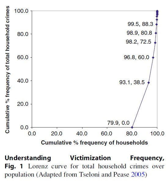
Figure 1 shows the Lorenz curve of the distribution of property crimes in England and Wales according to the 2000 British Crime Survey (BCS). The Lorenz curve is traditionally employed in public economics to describe how a society’s wealth is distributed across the population, and it is related to the Gini coefficient of income inequality. The closer the Lorenz curve is to the low right-hand corner of its square outline, the higher the inequality. In the extreme, one person holds all wealth or in this case experiences all crime.

Figure 1 shows that 80 % of households have not experienced any crime over the 1-year risk period used in the BCS. This is good news for the majority, but bad news for the minority. Tracking the Lorenz curve upward, it is seen that the 6.9 % of the most victimized households experience 61.5 % of crime in the sample. Further, the 3.2 % of such households experience 40 % of property crimes, and so on and so forth, until nearly 12 % of crimes affect the 0.5 % most heavily victimized households. This indicates that the crimes reported by the 20 % victimized households are allocated unequally. Figure 2 demonstrates this more clearly.

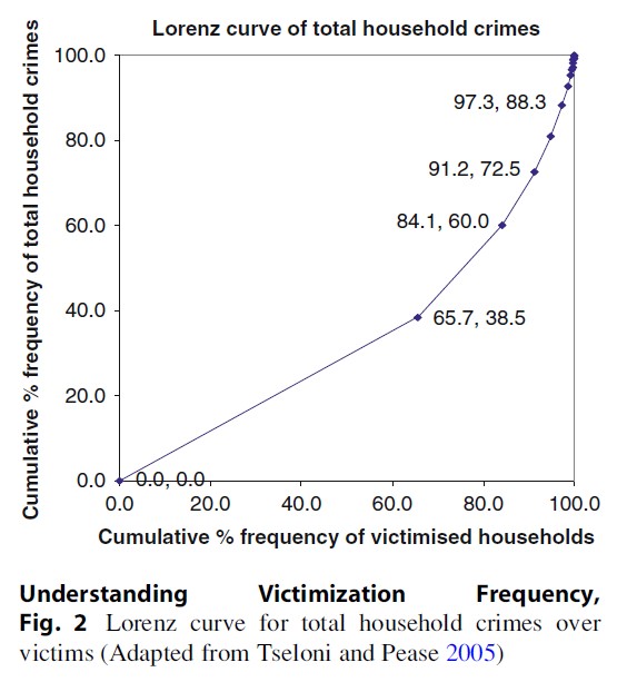
For instance, the least victimized 65.7 % of victims experienced 38.5 % of crimes (see Fig. 2). By contrast, the most victimized 2.7 % of victims experienced 11.7 % of crimes. Therefore, crime is affecting both the population and victims unequally. Assuming therefore an appropriate statistical model for highly skewed counts, the chances of two crimes (or any other given number) can be predicted (Osborn and Tseloni 1998).

As mentioned, a large portion of empirical victimization research looks at risk rather than the number of crimes per person. It thereby ignores repeat victimization which is an important component of high crime rates. This seems to be confirmed further by the significant reductions of repeat rather than single victimization rates (Thorpe 2007) during the last 15 or 20 years of considerable crime falls.

Measuring Repeat Victimization And Crime Concentration

Repeat victimization did not feature in a consistent manner in criminological research prior to the work by Ken Pease and colleagues in the 1990s (Forrester et al. 1990). With the exception of few still inspiring studies, such as Reiss (1980), a number of issues with regard to counting and analyzing crime incidents hindered the allocation of crimes over victims. For instance, the discontinuous nature of police statistics, which, as mentioned in the beginning, is offender-or at best location-centered, does not allow a straightforward victim-based aggregation. In addition, the infrequency of crimes overall, that is, in the general population (see Fig. 1), which becomes even more skewed when individual crime categories are analyzed, such as larceny or theft from the person, has led quantitative population-based victimization research to focus on the proportion of victims. Therefore, new ways to look into crime experiences were introduced (Farrell and Pease 1993).

Repeat victimization can be measured in a number of ways depending on the objectives of the analysis. The following fictional crime distribution of Table 1 demonstrates how. It assumes that 100 people were surveyed and a minimum of 0 and a maximum of 4 crimes were reported, the latter thankfully by just one respondent. The majority of hypothetical respondents (52) had no crime experience which gives a victimization risk of 48 %. But 18 respondents were repeat victims; therefore, the percentage of repeat victimization is 100 ×18/48, that is, 37.5 %. The total number of crimes is 75 which gives crime incidence of 75 % or 0.75 crimes per respondent. But crime concentration is 75/48, that is, 1.56 crimes per victim. Crime concentration should be distinguished from crime incidence which refers to the mean number of crimes in the entire population not just victims. Finally, 45 crimes are the result of repeat victimization; therefore, the percentage of repeat crimes is 100 × 45/75 which gives 60 %.

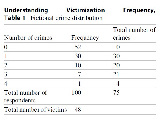
Ideally, therefore, examining the entire (skewed) distribution of crimes via compound Poisson statistical models that are appropriate for counts, such as the distribution given by the first two columns of Table 1, addresses both the binary victim/non-victim outcome that was the focus of early research and repeat victimization.

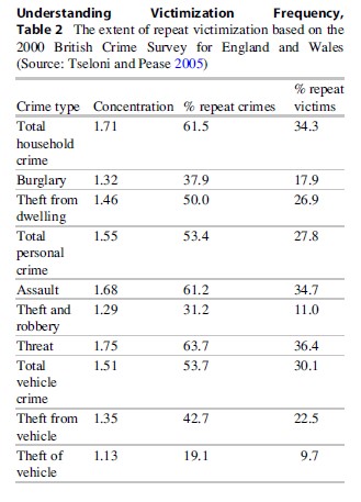
Table 2 shows the extent of repeat victimization for each crime type based on the 2000 BCS. “Concentration” measures the mean number of crimes per victim. The second column of “% Repeat crimes” shows the percentage of total crimes that affected the same victims. The last column, “% Repeat victims,” measures the percentage of victims who suffered at least two incidents by the respective crime type. For instance, threats and assaults are the most recurring individual crime types. Sixty-four percent of threats were against victims already threatened. Thirtysix percent of threat victims were threatened twice or more within a year. Evidently aggregate categories, such as total household or personal crime, have more repetition because a number of different offense-type counts and the boundaries between multiple and repeats are unclear.

Table 2 suggests that all crime types tend to be suffered disproportionately by the same targets. This is not limited to England and Wales. It is well established that repeats exist across crime types and cross-nationally with roughly similar victim characteristics (Farrell and Bouloukos 2000).

Why Is Crime Concentrated?

Having established that repeat victimization and crime concentration exist, the question calls for an answer. Why are individuals or households likely to experience more than one crime, especially when there are so many more non-victims in the population? Three explanations, which were conveniently borrowed from the literature on statistical analyses of accidents, have been suggested (Tseloni 1995). They are given below:

• Population heterogeneity (apparent contagion) – The simple fact that people are and behave differently and encounter dissimilar situations because they live and spend time in diverse places and/or settings. According to this explanation, all individuals have constant but unequal victimization risks. In the next section, the profile of individuals and settings which are vulnerable to crime and crime repetition is outlined.
• Event dependence (true contagion) – The chances of a second, third, and so on and so forth crime depend upon the outcome of the previous one. All individuals have the same initial risks, but these change after each victimization event. For instance, during his/her first attempt, an offender acquires more knowledge about the target. It is only natural that this new experience will inform and increase the chances of subsequent victimization of the same target.
• Spells – It is the time periods during which an unusually large number of crimes occur. For instance, burglars may operate in an area for a period of time and then move elsewhere perhaps being locked up or reformed. At the time of writing this, there is a spell of gold-related burglaries due to its increased price, for instance.

Traditional victimization theory and the majority of academic empirical research focus on the first explanation. Indeed, population heterogeneity has guided the prediction of the victim/non-victim dichotomy (please see the considerable work by Professors Lauritsen, Miethe, McDowall, and colleagues). The frequency of crime experience and victimization history is however ignored with few exceptions (for instance, Lauritsen and Davis-Quinet 1995), and as mentioned, it may not be a priority in terms of crime prevention as it is repeat crimes that contribute to high crime rates (Pease 1998). The second explanation, event dependence, has guided crime prevention by the Home Office in England and Wales since the 1990s and elsewhere (Pease 1998). The third explanation, spells, has hardly been explored to date (Bowers and Johnson 2005).

Predicting Victimization Frequency

In an oversimplified statement, which, as such, is open to legitimate criticism, victimization frequency depends on “who you are, where you live, and past crime experiences.” To be more precise, it can be predicted from the following:

• Individual risk and protective factors and their interactions
• The conditioning of the risk and protective factors according to context and
• The conditioning of the risk and protective factors according to victimization history

The various combinations of the above elements, given reliable victimization survey data and good statistical model fit, can tell how many times crime is expected to occur. The relative importance of each individual and contextual attribute as well as victimization history depends on the specific crime type examined. It has long been established that the mechanisms of victimization are better captured when focusing on narrower crime categories rather than aggregate crime types (Kennedy and Forde 1990). After modeling burglary incidence in England and Wales for almost two decades, the current author can safely say that, although the major risk and protective factors remain unchanged over time, their relative importance may change. Therefore, crime prevention practitioners and other readers should take the order of the independent effects given herein with a pinch of salt.

Independent Effects And Their Interactions

This section overviews the strongest (in terms of size of statistically significant effect) risk and protective factors associated with crime-specific victimization frequency. Perhaps not surprisingly, these effects are consistent both across periods and cross-nationally (Osborn and Tseloni 1998; Tseloni 2000; 2006). The following bullet points give the eight most important crime-specific factors. Eight is an arbitrary cutoff point (the full lists of risk and protective factors are available in the original studies). These are risk factors (indicated via R) which increase the mean number of crimes or protective (indicated via P) that reduce them. More than one attribute within the same bullet point implies that the effect sizes are effectively identical although the signs may be opposite, that is, presenting an (R) and a (P) along the same line.

The crime types overviewed here are total household and total personal crime (contrary to the writer’s own wisdom given in the previous section), burglary, household theft, and criminal damage.

The frequency of household crime can be predicted from the following:

• 3+ Cars (R)
• Lone parent (R)/prior assault (R)
• Inner city (R)/prior burglary (R)
• Social renting (R)
• Number of cars per household in the area (P)/terraced or town house (R)
• Percentage of 5–15 years old in the area (R)/area population density (R)/urban (R)
• Prior car theft (R)
• Over £30,000 household income (R)

The well-established opposite effect of individual and contextual affluence on victimization is demonstrated here. Area affluence, which is indicated by the average number of cars per household, is a protective factor against household crimes, while household affluence, given by the number of cars in the household and high income (Over £30,000), is a clear risk factor (Tseloni et al. 2002). Therefore, it seems that from a policy perspective, the relative well-off households in poor areas require more household crime protection than their neighbors which may contradict intuitive justice sentiments. In this vein, the relatively modest households living in affluent areas may consider themselves safe from being targeted.

The second fundamental lesson to be retained is that victimization history, even by a different crime type, as in the prior assault effect on aggregate household mean crimes above, is of high importance. Therefore, event dependence effects via the use of panel data, such as the NCVS, or questionnaire items about crime experiences that happened prior to cross-sectional surveys’ reference period are equally worth capturing as socioeconomic and contextual attributes (population heterogeneity).

Household crimes are disaggregated into burglary, household theft, and criminal damage – motor-vehicle crime is ignored here as it can happen away from the victims’ residence. The following set of bullet points shows the main factors associated with each crime type.

The frequency of burglary including attempts can be predicted from the following:

• 3+ Cars (R)/lone parent (R)
• Social renting (R)/prior burglary (R)
• Prior assault (R)
• Number of cars per household in the area (P)
• Prior car theft (R)/flat 2nd floor or above (P)
• 1–2 years in the area (R)
• Inner city (R)
• Percentage of 5–15 years old in the area (R) The best predictor for frequent burglaries is three or more cars in the household; the second and the third most important risk factors are again related to event dependence: been burgled and assaulted in the past (prior to the study period). To demonstrate the earlier point about crime definition-and period-specific effects, in analyses based on more recent BCS data, car ownership loses its top place in the set of associated factors to inner city/urban residence. In addition, when isolating burglary with entry from attempted burglary, a different order of the same set of risk factors appears (Tseloni 2011).

The frequency of household thefts can be predicted from the following:

• 3+ Cars (R)/lone parent (R)
• Prior assault (R)
• Social renting (R)
• Ethnic minority (P)
• Prior burglary (R)
• Terraced (R)
• Prior car theft (R)
• Nonmanual household reference person, henceforth HRP (R)

The following are most associated with the frequency of criminal damage:

• 3+ Cars (R)
• Prior assault (R)
• Percentage of 5–15 years old in the area (R)
• 1 or 2 cars (R)
• Terraced (R)
• Social renting (R)
• Number of cars per household in the area (P)/3 + adults in the household (P)
• Percentage of Indian-subcontinent household representative person (politically correct term for “head of household”) in the area (P)

As seen, for instance, the availability of young people in an area is the third most important factor for criminal damage but does not feature in the top eight factors for household theft and makes it last for burglary.

The risk and protective factors of personal crime are the following:

• Divorced (R)
• Single (R)
• Ethnic minority (P)
• 3+ Adults in the household (R)
• Social renting (R)/inner city (P)
• Private renting (R)/children (R)/flat (R)
• Area population density (R)
• Terraced (R)/over £30,000 household income (P)

Three things should be noted here. First, the ninth most important risk factor, which did not make it to the list, is area deprivation. Second, individuals’ affluence, ethnic minority, and living in inner city are protective factors for personal crimes. Third, gender is not within the eight (or nine) most associated factors. All three do not only appear in incidence analyses but replicate victimization risk results. Indeed, some studies have not evidenced any significant difference in personal victimization between men and women (Rountree et al. 1994), especially within households of high vulnerability (Tseloni 2000). If anything, females have higher chances of experiencing personal theft than males (Miethe and Meier 1990). Ethnic minorities are significantly less victimized by personal crimes than Whites overall (Tseloni 2000; Lauritsen 2001) and, in particular, when spending at least a night out per week, in full-time employment or study (Miethe et al. 1987) and within ethnically heterogenous communities (Rountree et al. 1994). More research is under way at the time of writing this both in the USA and the UK, but the traditional lifestyle theory propositions that males and/or ethnic minority individuals are more exposed and therefore victimized than others (Hindelang et al. 1978) seem to be counter-indicated by results of contextualized individual effects.

The frequency of victimization increases if households or individuals possess multiple risk factors. It diminishes if they possess risk alongside protective factors. In addition, some combinations of attributes reinforce victimization over and above the simple sum of the respective individual effects. For instance, in general, men are more frequently “threatened” than women. But divorced women experience triple the number of threats as divorced men (Tseloni 1995). Similarly, widowed people, who are in general the least victimized by personal crime marital status group, become disproportionally vulnerable in densely populated areas (Tseloni 2010). Therefore, context is as important as individual characteristics and lifestyle. The following section illustrates this point and the one after next explores it in more detail.

So What? How Practitioners Might Make Use Of Predicted Population Heterogeneity

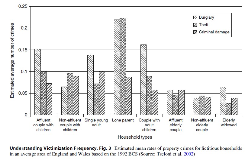
Figure 3 shows how estimated crime rates from empirical statistical models can provide information about the relative vulnerability of different households. Having this knowledge, group-specific crime prevention can be developed. For instance, a nonaffluent family experiences considerably more thefts than burglaries. Therefore, if this result is replicated, this group would benefit more from awareness about the risks of offering access into their house than from technological target hardening via burglary prevention devices. By contrast, a couple with adult children which probably possesses more valuables and gadgets would benefit from target hardening.

Figure 4 offers the same information as Fig. 3 but for risk rather than average victimization frequency. It is evident that notable differences exist between predicted risk and incidence. For instance, lone parents are at greater risk of burglary than theft but the mean number of respective events is similar. Single adults experience more incidents of criminal damage than theft but similar risks. This demonstrates that a different story might be told when risk and incidence are examined. By the same token, if interest centered upon victims of three or more repeats, a different order of specific-crime-type frequency per household composition might have appeared. Therefore, modeling (and predicting) the entire distribution of crimes offers flexibility in the choice of a cutoff point for analysis and intervention.

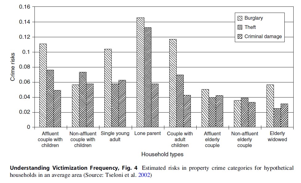
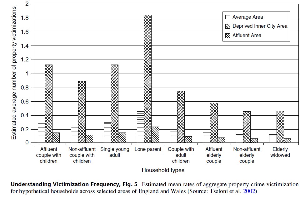
Figure 5 shows how the predicted household crime incidence over household types is influenced by area of residence. Even low vulnerability groups, such as a nonaffluent elderly couple, may experience more crimes in deprived inner city areas than the most vulnerable population subgroup, lone parents, in affluent areas. Therefore, context has a direct effect on victimization frequency. The next section discusses how it may also interact with and condition the individual and routine activity effects.

Conditioning Of Individual Factors According To Context And Victimization History

The interaction between individual and contextual characteristics, the so-called cross-cluster effect (Rountree et al. 1994; Tseloni 2006), addresses the following question: Why is person A more vulnerable than person B in a given situation but not always?

There are two types of cross-cluster interactions: explained, such as the area deprivation interaction with widowhood mentioned in the earlier subsection “Independent Effects and Their Interactions,” and unexplained or random. In the latter case, the importance of a risk or protective factor alters by context. It may jump up or down few places in the series of bullet point lists given earlier (subsection “Independent Effects and Their Interactions”) from one area to another. To illustrate this, please, consider the classic negative age effect on victimization. Figure 6 shows the average effect for England and Wales in 1999.

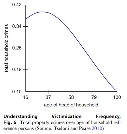
Age is indicated as the horizontal axis of Fig. 6. Household crimes (indicated in the vertical axis) increase for HRPs between the ages of 16 (the lower bound of the BCS sample at the time) and about 34 years old and then drop sharply as HRPs grow older. This curve however portrays the average of a wide range of age effects, such as seen in Fig. 7. Households with young HRPs experience about six times more household crimes in the “worse” area than in the best area. As they grow older, the number of household crimes they may experience converges regardless of where they live. As a result, ageing reduces victimization incidence more sharply in the “worst” area compared to the “good” ones.

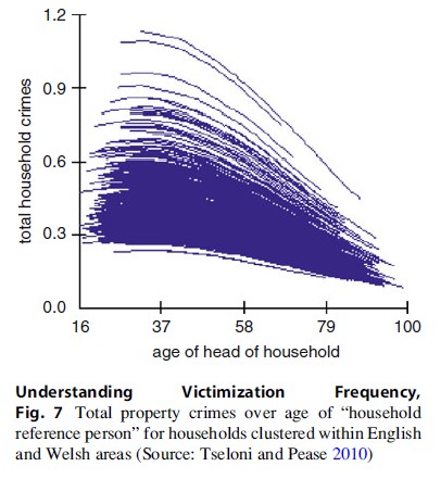
Another example is the lone parent risk factor: In “good” areas, lone parents are expected to experience roughly the same low number of household crimes as others, but in the “worst” area, they may experience roughly ten household crimes per year (Tseloni and Pease 2010). Similar conditioning of individual effects and lifestyle has been evidenced in victimization risk analyses especially, as mentioned in subsection “Independent Effects and Their Interactions,” with regard to ethnicity (Lauritsen 2001; Rountree et al. 1994).

The last issue in predicting crime concentration is to examine whether the effect of victimization history on current crime experiences depends on sociodemographic characteristics and lifestyle of individuals. To some extent, and especially during adjacent periods, when victims’ attributes and routine activities remain the same, event dependence is an indication of unmeasured population heterogeneity, namely, of subtle differences between people or households. The effects of recent victimization history in the short run are exacerbated by outgoing lifestyle and vary widely according to area of residence (Tseloni and Pease 2004).

Future Agenda

This essay discussed the acquisition of knowledge during the last two decades or so on victimization frequency and its prediction. In particular, crime risk and concentration can be examined simultaneously via crime count models and predicted from individual and contextual factors, victimization history, their interactions, and contextual conditioning.

That prediction will most definitely improve if population crime surveys:

• Incorporate a longitudinal element with data on the same households (rather than addresses as currently in the NCVS) that span longer than the 1-year reference period.
• Collect detailed information about each incident that occurred per victim.
• Locate as precisely as possible incidents on a timeline.

Given that crime concentration is predictable, it can also be prevented.

Bibliography:

1. Bowers KJ, Johnson SD (2005) Domestic burglary repeats and space-time clusters: the dimensions of risk. Eur J Criminol 2:67–92
2. Farrell G, Bouloukos AC (2000) A cross-national comparative analysis of rates of repeat victimization. Crime Prev Stud 12:5–25
3. Farrell G, Pease K (1993) Once bitten, twice bitten: repeat victimization and its implications for crime prevention. Crime prevention unit paper 46. Home Office, London
4. Felson M (2002) Crime and everyday life. Sage, Thousand Oaks
5. Forrester D, Frenz S, O’Connell M, Pease K (1990) The Kirkholt burglary prevention project: phase II. Crime prevention unit paper 23. Home Office, London
6. Hindelang MJ, Gottfredson MR, Garofalo J (1978) Victims of personal crime: an empirical foundation for a theory of personal victimization. Ballinger, Cambridge, MA
7. Kennedy LW, Forde DR (1990) Routine activities and crime: an analysis of victimization in Canada. Criminology 28:137–152
8. Lauritsen J (2001) The social ecology of violent victimization: individual and contextual effects in the NCVS. J Quant Criminol 17:3–32
9. Lauritsen JL, Davis-Quinet KF (1995) Repeat victimization among adolescents and young adults. J Quant Criminol 11:143–166
10. Miethe T, Meier R (1990) Opportunity, choice, and criminal victimization. J Res Crime Delinq 27:243–266
11. Miethe TD, Stafford MC, Long SJ (1987) Social differentiation in criminal victimization: a test of routine activities/lifestyle theories. Am Sociol Rev 52:184–194
12. Osborn DR, Tseloni A (1998) The distribution of household property crimes. J Quant Criminol 14:307–330
13. Osborn DR, Ellingworth D, Hope T, Trickett A (1996) Are repeatedly victimised households different? J Quant Criminol 12:223–245
14. Pease K (1998) Repeat victimization: taking stock. Crime detection and prevention series paper No. 90. Home Office, London
15. Reiss AJ (1980) Victim proneness in repeat victimization by type of crime. In: Fienberg S, Reiss AJ (eds) Indicators of crime and criminal justice quantitative studies. Department of Justice, Washington, DC, pp 41–53
16. Rountree PW, Land KC, Miethe TD (1994) Macro–micro integration in the study of victimization: a hierarchical logistic model analysis across Seattle neighborhoods. Criminology 32:387–414
17. Sampson RJ (2006) Collective efficacy theory: lessons learnt and directions for future inquiry. In: Cullen FT, Wright JP, Blevins L (eds) Taking stock: the status of criminological theory, advances in criminological theory, vol 15. Transaction Publishers, New Brunswick, New Jersey, pp 149–167
18. Shaw CR, McKay MD (1942) Juvenile delinquency and urban areas. Chicago University Press, Chicago
19. Thorpe K (2007) Multiple and repeat victimization. In: Jansson K, Budd S, Lovbakke J, Moley S, Thorpe K (eds) Attitudes, perceptions and risks of crime: supplementary volume 1 to crime in England and Wales 2006/7, Home Office Statistical Bulletin 19/07. Home Office, London, pp 81–98
20. Trickett A, Osborn DR, Seymour J, Pease K (1992) What is different about high crime areas? Br J Criminol 32:81–89
21. Tseloni A (1995) The modelling of threat incidence: evidence from the British Crime Survey. In: Dobash RE, Dobash RP, Noaks L (eds) Gender and crime. University of Wales Press, Cardiff, pp 269–294
22. Tseloni A (2000) Personal criminal victimization in the U. S.: fixed and random effects of individual and household characteristics. J Quant Criminol 16:415–442
23. Tseloni A (2006) Multilevel modeling of the number of property crimes: household and area effects. J R Stat Soc A Stat Soc 169(Part 2):205–233
24. Tseloni A (2010) ‘Individual and contextual risk factors of personal victimisation in England and Wales.’ Interdisciplinary workshop on ‘Urban social dynamics: inequalities, segregation and criminality’, EHESS, Paris. Available online http://cams.ehess.fr/ docannexe.php?id¼1011. Accessed 16 Nov 2010
25. Tseloni A (2011) ‘Household burglary victimization and protection measures: who can afford security against burglary and in what context does it matter?’ Crime Surveys Users Meeting, Royal Statistical Society, London. Available online http://www.ccsr.ac.uk/esds/ events/2011-12-13/index.html. Accessed 13 Dec 2011
26. Tseloni A, Pease K (2004) Repeat personal victimization: random effects, event dependence and unexplained heterogeneity. Br J Criminol 44:931–945
27. Tseloni A, Pease K (2005) Population inequality: the case of repeat victimization. Int Rev Victimol 12:75–90
28. Tseloni A, Pease K (2010) Property crimes and repeat victimization: a fresh look. In: Shoham S, Knepper P, Kett M (eds) International handbook of victimology. Taylor and Francis, Boca Raton, pp 127–149
29. Tseloni A, Osborn DR, Trickett A, Pease K (2002) Modelling property crime using the British Crime Survey: what have we learned? Br J Criminol 42:89–108
30. Tseloni A, Ntzoufras I, Nicolaou A, Pease K (2010) Concentration of personal and household crimes in England and Wales. Eur J Appl Math Spec Issue Math Models Crim 21:325–348

See also:

• How to Write a Research Paper
• Research Paper Topics
• Research Paper Examples

Free research papers are not written to satisfy your specific instructions. You can use our professional writing services to buy a custom research paper on any topic and get your high quality paper at affordable price.