Real Estate Economics Research Paper

This sample Real Estate Economics Research Paper is published for educational and informational purposes only. Like other free research paper examples, it is not a custom research paper. If you need help writing your assignment, please use our custom writing services and buy a paper on any of the economics research paper topics.

Real estate economics is the study of the markets for land and structures, including residential housing, commercial office space, and industrial warehouses. Although much theory has existed for decades regarding real estate markets, questions are being answered today regarding mortgage finance innovation, the rise of suburban business and residential centers, and the effects of zoning laws. The housing boom and bust of the first decade of the twenty-first century has meant that households, businesses, and governments have become more interested than ever in real estate and its effect on various aspects of the economy. In this research paper, the theory of real estate markets is first presented, including the relevance of real estate rental price, the heterogeneous nature of real estate, the importance of location, and the interaction with the macroeconomy. Next, various contemporary applications of real estate economics are discussed, followed by a description of government policy intervention in the real estate market. Finally, the housing boom and bust is presented along with areas for future research.

Theory of Real Estate Markets

Flow of Services, Rent, and Price

In many respects, real estate markets are similar to markets for other goods and services. There exist buyers who demand real estate by demonstrating a willingness and ability to pay for property. There are also sellers who supply real estate. One unique feature of real estate is that the goods in question—namely, land and structures—are long-lived. Consuming real estate does not result in the disappearance of the good as with, say, consuming a slice of pizza. Real estate can be purchased and enjoyed today and then sold again tomorrow. In fact, the vast majority of real estate sold in any year was previously owned. Because of this durability, the decision to buy or sell real estate must take a long time horizon into account.

Durable goods deliver a flow of services over time to the owner or user of that good. For example, a car lasts many years, and a car will deliver a flow of transportation services each year. Real estate delivers a flow of shelter services, in residential housing, and a flow of retail store space, in commercial real estate. The person who purchases a durable good takes current and all future flows of services into account when making the decision to purchase the good. This is true whether or not the buyer intends to use the services that flow from the durable good. For example, in the case of a car, although often the buyer intends to drive the car for a number of years after the purchase, car rental companies purchase large amounts of cars in order to charge rent to their customers. The same is true in real estate, where a large amount is owner occupied, while other people intend primarily to offer for rent the shelter or retail space to others. If the buyer intends to rent the real estate to others, then the buyer’s willingness to pay will be based on the rent that can be earned, which is determined by renters and landlords in the rental market for real estate. Renters will be willing to pay rent that is at or below the value that the renter puts on the flow of services. In fact, the dollar value of rent is an easy-to-obtain measure of the dollar value of the flow of services from a property.

Purchasing a piece of real estate today gives the buyer the use of services this year and every year in the future. See James Hamilton (2005) for a good discussion about how the buyer may approach the decision of whether to buy a house. The willingness to pay for that stream of service flows is equal to its present discounted value. The present discounted value is the sum of the discounted values, where the appropriate discount rate reflects the buyer’s opportunity cost of purchasing today. Typically, it is the mortgage interest rate, which may be adjusted for risk and taxes. Numerically, the present discounted value in year t, PDV„ is as follows:

where St is the flow of real estate services, i is the interest rate, and t is the year index. If the value of services grows at a constant rate g, and if g < i, then the above reduces to

real-estate-economics-research-paper-form2

The present discounted value will rise with the value of the flow of services provided by the property and the growth rate of services, and it will fall when the interest rate rises. This last result is because an increase in the interest rate will not only raise the numerator but also raise the denominator more, thus lowering the ratio. The present discounted value of the flow of current and future services is referred to as the fundamental value of real estate. The fundamental value simply says that the most that people will pay for a piece of real estate is the present discounted value of the flow of services. This is a very intuitive way to think about real estate pricing and shows the link between the market for real estate rentals and the market for real estate purchases—the main driver of real estate prices is the value that the end user puts on the property and the discount rate. The fundamental value of real estate is essentially an arbitrage condition that says that if the market price of real estate is equal to the present discounted value of future rents, then there are no sure profits to be made through buying or selling real estate, and thus, the market price of real estate will not rise or fall unless there is a change to the fundamental value.

Demand and Supply

The price of real estate in the short run is determined by supply and demand in the real estate market. See Denise DiPasquale and William Wheaton (1996, chap. 1) for a rigorous exposition of this material. The market for real estate, where potential buyers and sellers meet, is different from the market for rental properties, where renters and landlords come together to rent buildings. This discussion focuses on the market for rental properties and considers how that market sets the price and influences the construction, or development, of new real estate. In the rental market, each potential renter has an individual willingness to pay. The market willingness to pay is the sum of the willingness to pay for all renters, and just as with any good, the sum of willingness to pay determines the market demand for the good. As the market rental price of real estate falls, more and more renters will rent, and this results in the typical downward sloping demand curve, as shown by line Demand1 in Figure 59.1. Market demand is a function of the size and composition of the population, the local job market and incomes, local amenities, and other factors that are discussed later. Demand shifts come about when any of these factors change. The quantity or stock of real estate is fixed in the short run because it takes a relatively long time for new real estate to be built or developed, given permitting, zoning, and construction considerations. Figure 59.1 therefore shows supply, Supply1, in the rental market as a vertical line equal to the stock of real estate.

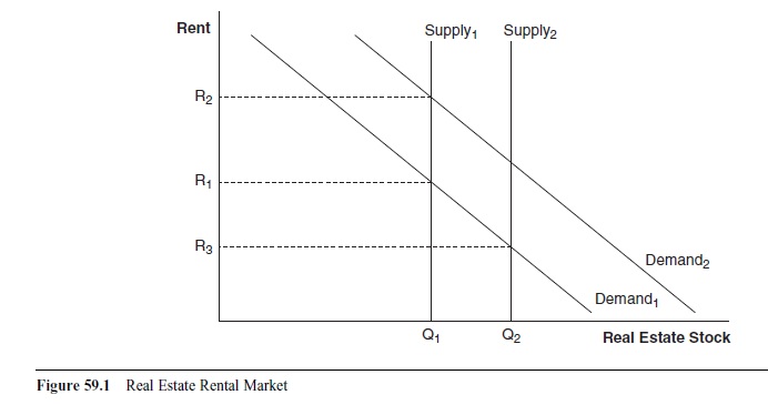Figure 59.1 Real Estate Rental Market

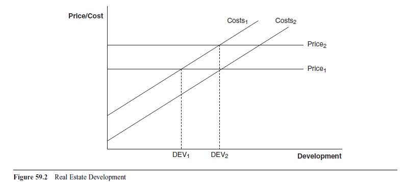Figure 59.2 Real Estate Development

Because real estate is long-lived, today’s supply is based on how much property was developed in the past. The amount of real estate construction or investment in any year depends on the availability and cost of funds for construction, on construction costs and technology, and on zoning considerations. Construction costs include fixed and marginal costs, and an increase in these costs will lead to less investment. Investment also depends on the price of real estate at the time that the investment decision is made. All else the same, a higher price of real estate will induce more construction and will lead to a higher future stock of real estate. If the price of real estate is above construction costs, then developers will find it profitable to build, but if the current price of real estate is below construction costs, then property will not be developed. Figure 59.2 shows how real estate development is determined. Given the price of real estate, there is one level of development that will be obtained. In Figure 59.2, if the price is equal to Pricej, and if costs are represented by line Costsp then real estate development is equal to DEVr If this new construction is greater than depreciation, which is the erosion of the real estate stock due to normal wear and tear, then the supply of real estate in the rental market will be greater next period. Real estate is just like any capital good in that the stock of real estate grows only if the investment flow is greater than depreciation.

There is one rental price at which the quantity of real estate supplied is equal to the quantity demanded, and that is the market clearing or equilibrium rent. In Figure 59.1, if the initial demand is represented by the line Demand1, and if the initial supply is represented by the line Supply1, then the initial equilibrium rent is R1. This current rent, along with the expected growth of rent and mortgage interest rates, will determine the present discounted value of future rents and the price that people are willing to pay to buy the real estate, and will it determine real estate development.

The equilibrium rent will change when demand or supply shifts. For example, suppose that population grows in a particular market. This will shift to the right the demand for real estate to Demand2, pushing up the rent to R2 in Figure 59.1. This increase in rent will lead to an increase in price to Price2 in Figure 59.2 and will lead to increased construction level DEV2. In the end, rent is higher, the price level is higher, and there is a larger stock of real estate. As another example, suppose that demand and price are back to their original positions and that credit becomes more easily available to developers. This will reduce construction costs to Costs2 in Figure 59.2 and increase investment to DEV2. The supply of real estate in Figure 59.1 will rise to Supply2, which lowers the rent to R3 and eventually lowers the price of real estate. In the end, the rent is lower, the price is lower, and there is a larger stock of real estate.

It is worth mentioning that although changes in the market price and the rental price of real estate are often positively correlated, as shown in the preceding two examples, one exception is when the mortgage rate changes. If the mortgage interest rate rises, this will decrease the present discounted value of future rents and lower the price. As a result, there will be less development, and the supply of real estate will fall in the rental market, which leads to higher rents.

Heterogeneity

Real estate is not a homogenous good in which each parcel of real estate is indistinguishable from another. Instead, each parcel has unique characteristics, including location, size, and amenities, and demand for these unique characteristics is determined in the market. The value for a particular real estate parcel is based on its unique characteristics. For example, people are generally willing to pay more to live near the ocean, and houses that are near the ocean have an ocean premium built into their market price. The more desirable features that a parcel has, the higher will be its market price. However, despite the uniqueness of each parcel, demand for a particular parcel is usually price elastic because other similar parcels are substitutes.

The demand and supply for a particular piece of real estate is composed of two distinct types of factors. The first is those characteristics that are unique to that parcel, such as exact location, number of rooms, size, land use zoning, and age of the structure. These unique characteristics will lead to different market prices among pieces of real estate. For example, commercial real estate that has better access to major road arteries will command a higher market rent and thus a higher market price, all else the same. But there are also factors that are common to all real estate within a certain market. In fact, one can define the market as all the real estate affected by these common factors. These common factors include the population, the local unemployment rate, and proximity to outdoor recreation activities, among others. These common factors will tend to raise or lower the market price of all properties but not change the relative prices. For example, if a large employer leaves the area, then this will decrease rents and lower the demand and prices for all real estate within the market.

Real Estate Value and Location

The theory of real estate value begins with the classic concept of Ricardian rent, which predicts that more desirable real estate will command a higher rent and market price as users compete for land. In the monocentric city model, distance to the single center of the city largely explains real estate prices. In urban residential real estate pricing, workers in a city must commute to their places of work, and they are willing to pay more for housing that is closer to their employers to avoid costs of commuting. Thus, land at the city center has a higher market price than land at the city edge. The price of all housing, which is made up of the price of the land and the price of the house, must be high enough to bid resources away from agricultural and physical structure uses. Thus, at the city edge, house prices must equal the sum of returns to agricultural land and construction costs of the house structure. But housing closer to the city center will have a higher price because people will pay to avoid the commute costs associated with greater distance from the city center. As commuting costs rise, prices in the city center rise relative to prices at the city edge. Users of urban land who differ based on their commuting costs, such as those with high wages and thus high opportunity costs of commuting time, will segregate themselves by location. Those with higher commuting costs will live closer to the city center, and if they earn higher wages, then segregation will appear along income levels. Because property closer to the city center has higher rent gradients associ-ated with it, builders will often increase density to substitute structure for land, and residential real estate closer to the city center will be more densely populated.

The original city center was often built decades or centuries earlier and often has very low density. Redevelopment of the city center into higher density use will become profitable for developers once residents feel that reduced commute costs are large enough to outweigh the dislike of higher density living.

This monocentric model of urban development has many shortcomings, as outlined in Alex Anas, Richard Arnott, and Kenneth Small (1998). The most visible is the fact that many of today’s cities are best described as multi-centered, with suburban city centers surrounding the original city core. Industrial land often occupies land on the edge of the city where land rent is cheaper and truck access to roads is good. Both industrial and commercial land has gathered in new outlying clusters within larger metropolitan regions. These alternative city centers compete with the traditional city hub for workers, and there has been much employment growth in these alternative suburban centers. A strong incentive to pull firms outside the central city hub is lower wages in the suburbs, where more and more of its workforce lives and where commuting times and thus wages are lower. Economies of agglomeration refer to the reduced costs to firms by clustering near one another. These include access to a large pool of skilled workers, better communication between firms, and closer proximity to suppliers. Counteracting this migration to the suburbs are increased costs of isolation and the reduction in agglomeration economies. At some point, the draw to an alternative city center is greater than the loss of the agglomeration effects, and the firm leaves the city center. One expects firms with the largest economies of agglomeration to locate in the large city center, while firms with less economies of agglomeration will be found in the alternative city centers. Recent increases in information technology, such as the Internet, may reduce the benefits to firms of clustering near one another, but Jess Gaspar and Edward Glaeser (1998) suggest that telecommunications may be a complement for face-to-face interaction and promote city center growth.

Commercial real estate can profit by locating near customers, suppliers, roadways, or mass transit terminals. Retailers would also like to cluster near complementary retailers because consumers try to minimize travel costs and the number of trips and often prefer to shop at a single shopping center. However, retailers would like to be located farther from similar retailers, because that increases their market power and pricing ability. Shopping malls give retailers the chance to cluster together in a central location, which may benefit some retailers, although some retailers, such as those who sell lower priced, nondurable goods that are purchased frequently are often not found in central shopping malls. Thus, rent for retail and commercial space is based partly on the mix of businesses in the area and the likelihood that those businesses will draw customers to the firm. See Eric Gould, B. Peter Pashigian, and Canice Prendergast (2005) for a recent discussion of shopping mall pricing.

The Macroeconomy and Real Estate

The real estate market is both a determinant of the regional macroeconomic climate and a product of that climate. Land and buildings are inputs into the production process, whether those markets are for industrial, commercial, or residential purposes, and real estate prices affect costs of production. Exogenous increases in the supply of real estate, perhaps from the opening of new lands for development, reduce rents and reduce costs to firms in the region, which gives those firms a cost advantage over other regions of the state or country. Employment and wages in the region will increase. A very inelastic supply of real estate can inhibit demand-driven economic growth if increases in housing prices raise the cost of living sufficiently to keep real wages from rising and attracting new workers into a region. Economy-wide factors, such as an exogenous increase in labor supply due to immigration, will affect the real estate market. Immigration will increase employment and production because wages and costs to firms fall, and it will increase the demand for real estate, which raises real estate rents. An increase in the demand for goods produced in the region will lead to an increase in the demand and price of all factors of production, including real estate. If the supply of real estate is price elastic, real estate prices will increase less and real estate development will be more than if real estate supply is inelastic. Local real estate markets depend on the national economy, with recessions typically reducing the demand for most types of real estate. But regional differences matter too, and a local real estate market may suffer relatively less during a recession if the relative demand for the particular mix of goods and services produced in the region does not fall. Finally, real estate wealth is a large fraction of total household wealth, and Karl Case, Robert Shiller, and John Quigley (2005) find large impacts of housing wealth on consumption.

Applications and Empirical Evidence

Hedonic Prices

Richard Muth (1960) wrote an early paper on hedonic pricing. A hedonic price equation relates the price of a piece of real estate to various characteristics of the property, such as distance to city center, size measured in square feet, number of bathrooms, and neighborhood quality, which can be measured as either low quality (0) or high quality (1). This is an attempt to resolve the issue that real estate is not a homogeneous good. The hedonic price equation decomposes real estate into various characteristics and estimates prices for each characteristic. In the case of residential housing, an example is as follows:

where a is a constant and the B s are the coefficients on each housing characteristic. Each B is the marginal impact of increasing the characteristic by one unit, in continuous variables such as distance, or the marginal impact of having that characteristic present, in binary characteristics such as neighborhood quality. One would expect that the coefficient on distance to the center of the city to be negative, because the amount of rent that people are willing to pay falls the farther the house is from the center of city, all else the same. One should note, however, that in very large metropolitan areas, some suburbs have developed into their own city centers, and distance to these new city centers may be just as important to house price as distance to the historic city center. James Frew and Beth Wilson (2002) present an empirical estimation of rent gradients in the multicentered city of Portland, Oregon. The coefficients on size, number of bathrooms, and neighborhood quality are expected to be positive because people are willing to pay greater rent for housing as these features increase, and thus, market real estate prices will be higher.

The coefficients in hedonic price equations are frequently estimated for both residential and commercial and industrial real estate parcels using ordinary least squares regression analysis or another estimation technique. There are typically many characteristics used to explain the price of real estate. In residential housing, these include local school quality, nearness to employment centers, proximity to amenities such as the ocean or recreational facilities, yard size, presence of a garage, and age of the house structure. In commercial or industrial property, these characteristics include nearness to major highways, airports, and rail lines; amount of pedestrian or car traffic; zoning considerations; nearness to suppliers, distributors, and customers; and parking availability, among others. loan Voicu and Vicki Been (2008) look at the effect of community gardens on property values in New York City and find a significant effect for high-quality gardens.

Demographics and Housing

The demand for residential real estate depends in the long run on characteristics of the population that move slowly over time. Gregory Mankiw and David Weil (1989) present a look at the implications of the baby boomers and the aging of the population on housing supply and demand. One factor is net household formation, which is the difference between newly created households and newly dissolved households in a year. A household, which is a group of related or unrelated individuals living at the same parcel of real estate, is a common unit of measurement by the Census Bureau. New households may be created when children leave their parents’ residence and through divorce, for example, while the number of households may fall during marriage and death, for example. The average size of households, as well as the age, composition, and income of households, will influence the typical features found in newly constructed housing, because developers quickly respond to current market conditions.

Age, income, demographic mobility, and marital status also greatly influence whether the household rents or buys housing. According to the 2007 American Housing Survey (U.S. Census Bureau, 2008), 31% of households rent the houses that they live in, 24% own the houses outright, and 44% are making mortgage payments. Renters are on average younger and have lower incomes than nonrenters. Permanent, or long-run average income, appears to influence the decision on whether to buy more than current income. Transaction costs of buying and selling a house are large, and renters move much more frequently than owners. Getting married and having children appear to be big factors that explain the switch from renting to owning.

Housing vacancies are a closely watched measure in the housing market. For a given level of sales, as vacancies rise, the average time on the market increases. Increased time on the market will tend to lower market prices, because sellers face increased opportunity cost of funds if they cannot sell their houses. New house builders will also be more motivated to lower prices, and they will also respond to greater average time on the market by reducing new construction. Although vacancy rates are typically studied at the local market level, consider the recent drop in U.S. new housing demand. The U.S. Census Bureau (2009) reports that the U.S. homeowner vacancy rate increased very quickly over 2006, averaging 2.375 in 2006 compared to 1.875 in 2005. New house sales fell from 1.283 million in 2005 to 1.051 million in 2006. In December of 2005, there were 515,000 new houses for sale, and the median time for sale was 4.0 months, while in December of 2006, there were 568,000 new houses for sale, and the median time for sale was 4.3 months. The median price of new houses continued to rise for 2 more years, until falling from $247,900 in 2007 to $230,600 in 2008. Builders responded to these market changes, and from 2005 to 2006, housing starts fell from 2.068 million to 1.801 million units.

Mortgage Financing

Residential real estate typically sells for hundreds of thousands or even millions of dollars. This is greater than most households’ annual incomes. Households typically do not save over many years to purchase housing but rather obtain financing to purchase residential real estate. Financing terms have changed considerably over the last 10 years and continue to change. Except for a short number of years in the first decade of the 21st century when houses could be bought with little or no down payment, down payments of 20% are common on loans. The down payment is subtracted from the sum of the purchase price and all fees and expenses to determine how much the buyer must finance. A mortgage is a residential real estate loan with the real estate itself as collateral. Most mortgages are fully amortizing, which means that the principal balance is repaid over the life of the loan, which is usually 30 years but sometimes more or fewer, such as 40 or 15 years. A common question asked is why does the principal balance decline very slowly in the first years of the loan? To answer this, it is helpful to think of a mortgage as a loan that is to be repaid every month. After the first month of the loan, the interest due is extremely large, because the outstanding principal is large. As the number of months goes by, the interest due becomes less because the principal is being paid down. In the final months, the interest due is small because the principal is small.

Many residential mortgages do not have fixed mortgage interest rates over the lives of the loans but rather have a rate that rises and falls, within limits, along with the prevailing interest rate. These adjustable rate mortgages (ARMs) became more popular with lenders after the high inflation of the 1970s, when lenders were paying high interest rates on short-run liabilities (deposits) while receiving much lower interest rates on long-term assets (loans). Another recent change to mortgages has been the use of mortgages that do not fully amortize. These interest-only and even negative-amortizing loans allow the monthly mortgage payments to vary, within limits, such that the loan principal balances do not fall as they would with fully amortized loans. These pick-a-payment mortgages usually require full amortization to begin a few years after the loan begins.

Funding for mortgages is typically provided by commercial banks and thrifts, and these institutions, as well as mortgage brokers, typically issue mortgage loans to households. However, it is very common for these loans to be quickly sold on the secondary mortgage market to pension funds, insurance companies, and other investors. Mortgage-backed securities (MBSs) or mortgage bonds are sold to investors. Investment banks and the government-sponsored enterprises Fannie Mae and Freddie Mac package individual mortgages into these securities, which are sold on huge markets. The pooling of individual mortgages can reduce risk because only a small number ofborrowers are expected to default. Fannie Mae and Freddie Mac also guarantee the payments on the securities that they process. Mortgages that conform to Fannie Mae and Freddie Mac standards, such as maximum loan to value, make up most of the secondary market, and the standardization of loans has allowed the market for these securities to grow. Conforming mortgage loan amounts must be below a threshold limit, adjusted to take average market price into account, or else the loans may be classified as jumbo loans, which have higher interest rates.

Government Policy

Tax Treatment of Housing

The federal government provides incentives to purchase housing to encourage home ownership. Government intervention is often justified on the grounds of positive externalities that result from home ownership, such as the idea that home owners will better maintain the exterior appearance of their houses than home renters or landlords. Glaeser and Jesse Shapiro (2003) lead an excellent discussion about the positive and negative externalities associated with home ownership. The mortgage interest deduction, whereby interest payments (not principal payments) are tax deductible, cost the federal government $67 billion in 2008, according to the Joint Committee on Taxation (2008). Additionally, local property taxes are deductible for federal income taxes. The marginal benefit to the owner of these tax deductions is equal to the deduction multiplied by the marginal tax rate. Because federal taxes allow a standard deduction, the housing tax incentives are relevant only if the household itemizes, but low- to moderate-income households often do not itemize. The evidence shows that federal tax treatment of housing has a more powerful effect in encouraging people to purchase larger houses rather than to purchase housing for the first time. Other tax incentives include a large exemption on housing capital gains and the mortgage interest deduction for state income taxes in many states. According to the Legislative Analyst’s Office (2007) in California, the largest California income tax deduction is the mortgage interest deduction, which cost $5 billion in reduced revenue in 2007 to 2008. Various distortions are created by state tax treatment of housing, such as Proposition 13 in California, which discourages sales of existing houses because property taxes tend to be lower the longer one resides at an address.

Retail Development

In many towns, the location of newly developed retail space is a very sensitive political matter that often requires a vote by the city council or a voter referendum. This is because of the impact of new retailers on the sales of existing retailers. If a new shopping center is built, existing retailers will often lose sales and market pricing power. Of course, the total amount of retail sales may remain unchanged, with the new shopping mall simply taking sales from existing business, and sales in one town may rise at the expense of sales in a nearby town. In rural communities, a new shopping center may divert sales away from out-of-the-area retailers or Internet retailers. The rise of Internet retailing can reduce the overall demand for retail real estate while increasing the demand for warehouse real estate. It remains to be seen how demand for retail space, and retail rental prices, will be affected in the long run by the rise in Internet retailers. Elaine Worzala and Anne McCarthy (2001) present an early examination of Internet retailing on traditional retail location.

Zoning

Municipalities, counties, and special local governments, such as water districts, Indian tribes, and coastal commissions, set property tax rates and zone land for specific uses. They use this tax revenue and grants from the federal and state governments to administer public expenditures on items such as schools and infrastructure. These local governments usually have a much larger impact on real estate markets than do the federal and state governments. In the classic Tiebout model, the difference in spending levels by communities on public services, such as school quality and police protection, reflects differences in community preferences. Communities that value higher quality schools will spend more on school services than those communities that do not, and residents will segregate into locations that reflect differences in willingness to pay for public services. Because willingness to pay often depends on income, differences in public expenditures will also reflect differences in average income across communities.

When considering new land development for either residential or commercial purposes, local governments will ask whether the new development will make existing residents better or worse off. If the new development requires on average less expenditure and raises more in property taxes compared to existing developed land, then current residents will be better off. On the other hand, if the new development requires more expenditure and raises less in property taxes on average compared to existing development, then current residents will not be in favor of development. Property taxes are based on land value and are not directly proportionate to the number of households on a parcel. It is therefore likely that compared to existing housing, denser housing development will generate a demand for public services that is greater than the higher property tax revenue collected. As a result, many localities require a minimum lot size, which has the effect of keeping communities segregated by lot size and income.

Commercial and industrial real estate is also zoned by local governments. The big concern with nonresidential development is the impact on the character of the community. Households typically want to live near other households or amenities such as parks and prefer to not live near commercial or industrial sites. This is one reason property taxes tend to be set higher for nonresidential uses. Towns that are more willing to accept new tax revenue in exchange for an altered community character are more likely to have nonresidential real estate developed within their jurisdictions.

Zoning authority is typically justified by the externalities that land use imposes on other individuals in the market and by the need to provide public goods. Of course, zoning is a much-debated political matter, and there is no doubt that in practice, zoning considerations are often made that redistribute resources rather than improve the quality of living for citizens. Zoning will restrict the supply of new development and raise real estate prices. Glaeser and Joseph Gyourko (2003) find that in U.S. regions where zoning is more restrictive, such as coastal states, high housing prices are the result. Negative externalities resulting, for example, from industrial pollution, noise, odor, dilapidation, and increased parking congestion, can adversely impact residential, commercial, and industrial real estate values. Positive externalities such as brown field restoration or regular exterior house maintenance can increase real estate values. Transaction costs tend to make an optimal private market solution in the presence of externalities difficult to obtain, and a common economic solution is government intervention. Local governments extensively control or restrict land use to alleviate externalities. For example, a large city might require newly constructed apartments to have at least one on-site parking space per residential unit to reduce street parking congestion. Governments also turn toward market incentives that internalize the external costs, such as a large city charging car owners a fee for on-street parking permits. Another example of a serious negative externality from real estate is traffic congestion. Users of residential, commercial, and industrial real estate drive on existing road-ways and can create substantial gridlock, especially at rush hour. This increases travel time for users, and estimates of the aggregate value of time lost can be substantial.

The City of London recently implemented a traffic congestion charge on cars during business hours, and the effect has been a substantial drop in congestion. Public goods, which once created are nonexcludable, face the well-known free-rider problem, which predicts underprovision of the good. Public goods include roads, parks, and footbridges. Local governments often zone real estate to provide for open space or tax residents to pay for road maintenance, for example. Richard Green (2007) finds that airports can help a region to experience economic growth. The optimum land use and government response to externalities and public goods will change over time. However, existing real estate usage is based on historical decisions, because real estate structures are typically long-lived, and governments may need to periodically revisit land use zoning.

Real Estate After 2000 and Future Directions

Housing Boom and Bust

Residential real estate prices began to climb very quickly in the early 2000s in many countries across the globe, and starting around 2006, prices began to decline. In the United States, nominal prices climbed 90% as measured by the Case-Shiller Index. The Case-Shiller Index is a repeat sales price index, which calculates overall changes in market prices by looking at houses that sold more than once over the entire sample period to control for differences in quality of house sold. In some regions, the median selling price of a house doubled in about 3 years from 2002 to 2005. Although regional real estate markets had previously experienced quick price increases, such as the Florida land boom of the 1920s, by all accounts this was the fastest increase in housing prices at the aggregate national level ever. As Shiller (2007) shows, inflation-adjusted U.S. housing prices were remarkably consistent since 1890, with the 1920s and 1930s being the exception of years of low prices. But since the late 1990s, housing prices in the United States on average grew to levels not seen in any year in which data are available. This fast rise in house prices encouraged a great deal of investment into both residential and commercial real estate. Construction employment soared, as did the number of people working as real estate agents and mortgage brokers. By 2008, housing prices had fallen 21% from their peak levels, which was a greater fall, in inflation-adjusted terms, than during the Great Depression. Accompanying this massive drop in prices was a fall in new and existing house sales, an increase in foreclosures to record levels, a drop in construction spending and commercial real estate investment, massive drops in government tax collections, and a huge drop in jobs in construction, real estate, and the mortgage industry. Mortgage companies, banks, and financial firms that held real estate assets shut their doors, and there was massive contraction and consolidation in these industries. The U.S. recession that began in 2007 accompanied the collapse of the housing market.

It is important to explain both the boom and the bust of this historic housing cycle. Cabray Haines and Richard Rosen (2007) compare regional U.S. housing prices and find evidence that actual prices rose above fundamental values in some markets. The boom can be partly explained by the fact that mortgage interest rates were very low at the onset, which according to the fundamental value approach should raise house prices because lower interest rates will raise the present discounted value of future rents. But it seems that changes in mortgage financing may have been an even more important part of the explanation, and many economists characterize the housing boom as a manifestation of a credit bubble that saw simple measures such as the price-to-rent and price-to-income ratios rise to levels above historic averages. Housing affordability fell sharply in most of the country. The use of MBSs increased, and mortgage lenders greatly reduced holdings of their mortgages in the so-called originate-to-distribute model. Mortgage lending standards fell as more and more people fell into the subprime (poor credit history) or Alt-A (high loan to income value) borrowing categories and down payment and income documentation requirements were greatly reduced.

Both this increase in supply and the increase in demand for mortgage credit increased the demand for houses, which pushed prices to record highs. Starting in 2006, and particularly in 2007, the appetite for MBSs fell greatly as mortgage defaults increased across the country. The drop in available mortgage credit was a blow to new buyers, those refinancing, and those seeking to trade up or purchase second houses. The result was a huge drop in demand for housing. The U.S. Census Bureau (2009) reports that in the fourth quarter of 2008, the home ownership rate was 67.5%, the same level as the fourth quarter of 2000.

The Federal Reserve’s (2009) Flow of Funds Accounts report that household percentage equity was lower than at any time in over 50 years of data. Government reaction to the housing bust has been unprecedented. In 2008, the U.S. Treasury Department and the U.S. Federal Reserve Bank tried to encourage consumer confidence in financial markets, brokered mergers between insolvent institutions and other companies, and committed hundreds of billions of dollars to help the financial industry and the U.S. economy at large. In September of 2008, Fannie Mae and Freddie Mac were placed into government conservatorship when their stock prices plummeted and they were unable to raise capital. A flurry of legislation passed that reduced income taxes for home buyers. At the federal level, first-time homebuyers in 2008 who were below the income limit received a credit on their taxes up to $7,500, which must be repaid over 15 years, while in 2009, there was a refundable tax credit equal to 10% of the purchase price of the house, up to $8,000. In California, a non-means-tested tax credit of 5%, up to $10,000, was available to all purchasers of newly constructed houses. Other states had their own home buyer income tax credits.

Areas for Future Research

One of the challenges of future research will be to better understand how financial product innovation contributed to the housing boom and what types of regulation would best fend off a similar future boom and bust cycle. Chris Mayer, Karen Pence, and Shane Sherlund (2008) point to zero-down-payment financing and lax lending standards as important contributors to the dramatic increase in foreclosures. Additionally, the difficulty of modifying mortgages and approving sales for a price lower than the outstanding principal balance (short sales) became evident with the diffuse ownership of mortgages through MBSs. In 2006, the Chicago Mercantile Exchange started issuing home price futures contracts with values based on the Case-Shiller Index for select cities. Like any futures contract, these are agreements between sellers and buyers to exchange housing contracts in the future at predetermined prices. If at the future date the actual contract price is higher than the agreed-upon price, then the buyer of the futures contract profits, while if at the future date the actual contract price is below the agreed-upon price, then the seller of the futures contract profits. An owner of residential real estate can use futures contracts to protect or hedge against price risk. For example, if the market price of a house falls, then the owner has a drop in net wealth. However, if an individual had sold a home price futures contract, then he or she may have earned a profit that cancelled the loss of owning housing. The ability of individuals, investors, and developers to protect themselves against price risk had been very limited before the introduction of these S&P/Case-Shiller Home Price futures, and it remains to be seen how well used these futures contracts will be.

Mark Bertus, Harris Hollans, and Steve Swidler (2008) show that the ability to hedge against price risk in Las Vegas is mixed.

An active literature has grown regarding housing and the labor market. Andrew Oswald (1996) shows that across countries, home ownership rates and unemployment rates are positively correlated. Jakob Munch, Michael Rosholm, and Michael Svarer (2006) find evidence that geographic mobility is decreased with home ownership, but home ownership appears to reduce overall unemployment. With more and more people having mortgage principals greater than the current market value of their houses, it seems that job mobility and wages will be negatively impacted.

Conclusion

This research paper reviewed the theory of real estate markets, including the important relationship of real estate rental price to selling price. Location is a key determinant of real estate rental price, but every parcel of real estate is unique, and hedonic pricing can determine the value that users place on individual characteristics of real estate. Most real estate is purchased with borrowed funds, and there have been important changes in mortgage financing over the last decade. The government treatment of real estate through taxation and zoning or land use restrictions will continue to be an important policy topic in the future. But perhaps the most visible issue in the short run is the impact of the real estate boom and bust. Future research will undoubtedly try to determine whether government policy can effectively prevent or mitigate the effects of similar episodes in the future.

Bibliography:

- Anas, A., Arnott, R., & Small, K. A. (1998). Urban spatial structure. Journal of Economic Literature, 36(3), 1426-1464.
- Bertus, M., Hollans, H., & Swidler, S. (2008). Hedging house price risk with CME futures contracts: The case of Las Vegas residential real estate. Journal of Real Estate Finance and Economics, 37(3), 265-279.
- Case, K. E., Shiller, R. J., & Quigley, J. M. (2005). Comparing wealth effects: The stock market versus the housing market. B. E. Journals in Macroeconomics: Advances in Macroeconomics, 5(1), 1-32.
- DiPasquale, D., & Wheaton, W. C. (1996). Urban economics and real estate markets. Englewood Cliffs, NJ: Prentice Hall.
- Federal Reserve. (2009). Flow of funds accounts of the United States. Available at http://www.federalreserve.gov/releases/ z1/current/z1.pdf
- Frew, D., & Wilson, B. (2002). Estimating the connection between location and property value. Journal of Real Estate Practice and Education, 5(1), 17-25.
- Gaspar, J., & Glaeser, E. L. (1998). Information technology and the future of cities. Journal of Urban Economics, 43(1), 136-156.
- Glaeser, E. L., & Gyourko, J. (2003, June). The impact of building restrictions on housing affordability. Economic Policy Review, 21-29.
- Glaeser, E. L., & Shapiro, J. M. (2003). The benefits of the home mortgage interest deduction. Tax Policy and the Economy, 17, 37-82.
- Gould, E. D., Pashigian, B. P., & Prendergast, C. J. (2005). Contracts, externalities, and incentives in shopping malls. Review of Economics and Statistics, 87(3), 411-422.
- Green, R. K. (2007). Airports and economic development. Real Estate Economics, 35(1), 91-112.
- Haines, C. L., & Rosen, R. J. (2007). Bubble, bubble, toil, and trouble. Economic Perspectives, 31(1), 16-35.
- Hamilton, J. (2005). What is a bubble and is this one now? Econ browser. Retrieved December 28, 2008, from http://www.econbrowser.com/archives/2005/06/what_is_a_bubbl.html
- Joint Committee on Taxation. (2008). Estimates of federal tax expenditures for fiscal years 2008-2012 (JCS-2-08). Washington, DC: Government Printing Office.
- Legislative Analyst’s Office. (2007). Tax expenditures reviews. Available at http://www.lao.ca.gov/2007/tax_expenditures/tax_expenditures_1107.aspx
- Mankiw, N. G., & Weil, D. N. (1989). The baby boom, the baby bust, and the housing market. Regional Science and Urban Economics, 19, 235-258.
- Mayer, C. J., Pence, K. M., & Sherlund, S. M. (2008). The rise in mortgage defaults (Finance and Economics Discussion Series Paper No. 2008-59). Washington, DC: Board of Governors of the Federal Reserve System.
- Munch, J. R., Rosholm, M., & Svarer, M. (2006). Are homeowners really more unemployed? Economic Journal, 116, 991-1013.
- Muth, R. F. (1960). The demand for non-farm housing. In A. C. Harberger (Ed.), The demand for durable goods (pp. 29-96). Chicago: University of Chicago Press.
- Oswald, A. (1996). A conjecture of the explanation for high unemployment in the industrialised nations: Part 1 (Research Paper No. 475). Coventry, UK: Warwick University.
- Shiller, R. J. (2007). Understanding recent trends in house prices and home ownership (NBER Working Paper No. 13553). Cambridge, MA: National Bureau of Economic Research.
- S. Census Bureau. (2008, September). American housingsurvey for the United States: 2007. Available at http://www.census .gov/prod/2008pubs/h150-07.pdf
- S. Census Bureau, Housing and Household Economic Statistics Division. (2009). Housing vacancies and home-ownership. Available at http://www.census.gov/hhes/www/ housing/hvs/historic/index.html
- Voicu, I., & Been, V (2008). The effect of community gardens on neighboring property values. Real Estate Economics, 36(2), 241-283.
- Worzala, E., & McCarthy, A. M. (2001). Landlords, tenants and e-commerce: Will the retail industry change significantly? Journal of Real Estate Portfolio Management, 7(2), 89-97.
Free research papers are not written to satisfy your specific instructions. You can use our professional writing services to buy a custom research paper on any topic and get your high quality paper at affordable price.
ORDER HIGH QUALITY CUSTOM PAPER
Always on-time
Plagiarism-Free
100% Confidentiality