Observational Epidemiology Research Paper

This sample Observational Epidemiology Research Paper is published for educational and informational purposes only. If you need help writing your assignment, please use our research paper writing service and buy a paper on any topic at affordable price. Also check our tips on how to write a research paper, see the lists of health research paper topics, and browse research paper examples.

Introduction

Observational epidemiologic studies are those in which an investigator observes what is occurring in a study population without intervening. In an observational study addressing the question of whether physical activity protects against coronary heart disease, an investigator might note at the beginning of a study, and at intervals throughout the study, the physical activity level of the study participants and relate this to the development of coronary heart disease. This contrasts with an experimental (or intervention) study, in which the investigator assigns study participants, preferably at random, either to be exposed or not to be exposed to a particular agent or activity. For instance, an investigator would randomly assign some people to a physical activity enhancement program and others not to be in this program, and then follow them up for development of coronary heart disease. Because of the randomization process, on average those assigned to the physical activity program will otherwise be similar to those assigned to the comparison group. In observational studies, however, physically active individuals might tend to differ in many other ways from inactive individuals. Thus, observational studies, which are the subject of this research paper, present special challenges when used to learn about disease causation.

Some Uses Of Observational Epidemiology

One use of observational studies is to determine the magnitude and impact of diseases or other conditions in populations or in selected subgroups of the population. Such data are useful in setting priorities for investigation and control, in deciding where preventive efforts should be focused, and in determining what type of treatment facilities are needed. Observational studies can be used to learn about the natural history, clinical course, and pathogenesis of diseases. Observational studies may be used to evaluate the effectiveness of therapeutic procedures or new modes of health-care delivery, although randomized trials are usually the preferred method of study for such evaluations. Most commonly, observational epidemiologic studies are used to learn about disease causation, and this application of epidemiology will be emphasized in this research paper.

Descriptive Studies

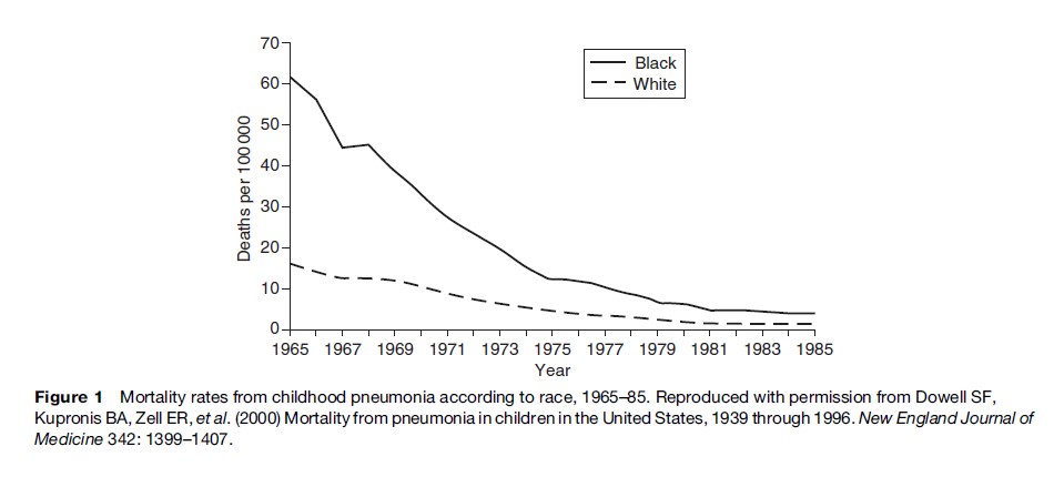
Descriptive studies generally provide information about the distribution of diseases and other characteristics without testing specific hypotheses about causation. Often such studies are used to generate hypotheses about causation. Many descriptive studies provide information on patterns of disease occurrence in populations according to such attributes as age, gender, race/ethnicity, marital status, social class, occupation, geographic area, and time of occurrence. Routinely collected data from such sources as cancer registries, death certificates, hospital discharge records, other medical records, and general health surveys are generally used for descriptive studies. This information can be used to indicate the magnitude of a problem or to suggest preliminary hypotheses about disease causation. For instance, in a classic descriptive epidemiologic study, maps of mortality rates of site-specific cancers by county in the United States (Mason et al., 1975) showed that certain geographic areas had particularly high or low mortality rates, suggesting that specific industries or other geographic factors might be responsible for the high rates. In another example, mortality rates from pneumonia in children in the United States have declined markedly since 1939. The steep decline in mortality rates in black children from 1966 to 1982 (Figure 1) is hypothesized to have resulted from improved access to medical care for poor children (Dowell et al., 2000).

Other types of descriptive studies are case reports and case series. In a case report, one person with a certain disease and certain exposure is noted. For instance, suppose one young woman with pulmonary embolism is observed to be using oral contraceptives. This one case obviously does not prove that use of oral contraceptives increases the risk for pulmonary embolism, but it might suggest that the possibility of such an association should be considered in more rigorous studies because pulmonary embolism is very rare among young women. In a case series, exposures in several cases with a given disease are noted. A physician might observe that eight out of ten young women with pulmonary embolism were using oral contraceptives at the time the embolism occurred. While 80% may seem a high percentage, oral contraceptives are widely used by young women, and it might be that eight out of ten young women randomly selected from the general population use oral contraceptives. Thus, a case series generally does not provide definitive information because a comparison (or control) group of young women without the disease is needed to determine if the 80% figure is in excess of expectation. In a case series from an outbreak of severe viral encephalitis associated with Nipah virus in Malaysia (Goh et al., 2000), some 93% of cases reported direct contact with pigs, usually in the 2 weeks before the onset of the illness. This high percentage is strongly suggestive of transmission from pigs to humans, but a properly designed case-control study (to be described in the next section) would be needed to show this more definitively. A case series of eight patients with vitamin D intoxication in the Boston area was sufficient to indicate that a local dairy was incorrectly and excessively fortifying its milk with vitamin D ( Jacobus et al., 1992). In this instance, no comparison group was needed, because even one case was sufficient to raise concern.

Nevertheless, case reports, case series, and other descriptive studies are usually useful only in providing leads for studies designed specifically to test hypotheses. Such hypothesis-testing studies are often referred to as analytic epidemiologic studies.

Analytic Studies

Analytic epidemiologic studies are designed to test causal hypotheses that have been generated from descriptive epidemiology, clinical observations, laboratory studies, and other sources, including analytic studies undertaken for other purposes. Analytic studies seek to determine why a disease is distributed in the population in the way it is. Because analytic studies often necessitate the collection of new data, they tend to be more expensive than descriptive studies, but, if properly designed and executed, generally allow more definitive conclusions to be reached. Common types of analytic observational studies include case-control, cohort, and cross-sectional studies, as well as some hybrid designs. Ecologic studies will also be briefly described. Although these analytic study designs usually provide more definitive information than descriptive studies, in some instances experimental studies may be needed to demonstrate causality.

Case-Control Studies

These are studies in which the investigator selects persons with a given disease (the cases) and persons without the given disease (the controls). Certain characteristics or past exposure to possible risk factors (e.g., cigarette smoking) in cases and controls are then determined and compared.

Cases are typically people seeking medical care for the disease. Usually only newly diagnosed cases are included in order to be more certain that the risk factor preceded the disease rather than being a consequence of the disease, and so that cases of short duration are appropriately represented.

A useful working concept of a control group has been given by Miettinen (1985): The controls should be selected in an unbiased manner from those individuals who would have been included in the case series if they had developed the disease under study. Thus, the optimal control group depends on the source of the cases, but the relative costs of obtaining the various types of controls and the resources available to the investigator are also taken into account in selecting control groups. Sometimes controls are matched to cases on certain important characteristics such as age and sex (see section titled ‘Confounding variables’). These characteristics can also be taken into account in the statistical analysis if no matching was done at the outset or if matching was not fine enough.

If the cases consist of all people developing the disease of interest within a defined population, then the best single control group would usually be a random sample of individuals from the same source population who have not developed the disease. In the United States, controls are frequently identified through random-digit dialing to members of the same community from which the cases arose. In countries with population registries, controls are typically selected from the registries. If cases come from a defined group such as members of a health maintenance organization, controls are generally sampled from among other members of the health maintenance organization.

In a case-control study of the possible protective effect of phytoestrogen consumption against the development of breast cancer (Horn-Ross et al., 2001), breast cancer cases were ascertained from the Greater Bay Area Cancer Registry, which includes all cases of newly diagnosed cancer among residents of the Greater Bay Area. Controls were identified through random-digit dialing of telephone numbers in the same area. A case-control study of the association between blood transfusions and non-Hodgkin’s lymphoma (Maguire-Boston et al., 1999) ascertained all cases diagnosed among Olmsted County, Minnesota, residents at the two medical-care providers in the county (Mayo Clinic and Olmsted Medical Center) and sampled controls from other Olmsted County residents who had been enumerated in a special census.

If cases are identified at certain hospitals that do not cover a defined geographic area, it is usually impossible to specify the source population from which the cases arose. In this instance, controls are often chosen from among patients with other diseases admitted to the same hospitals as the cases, since one wants to obtain a source of controls subject to the same selective factors as the cases. It is usually desirable to include as controls people with a variety of other conditions, so that no single disease is unduly represented in the control group. Generally, it is important to exclude potential controls who have had their disease for a long period of time because, like the cases, the presence of their disease may have influenced their exposure to possible risk factors. Such characteristics as physical activity, diet, weight, and medication use may change as a result of many diseases.

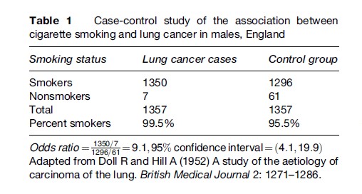
The classic case-control studies of Doll and Hill (1952) of the association between cigarette smoking and lung cancer (see Table 1) identified cases from several hospitals in England and chose as controls patients admitted to the same hospitals with other diseases who had a similar age and sex distribution to the cases. Although cigarette smoking was very common among both cases and controls, a higher percentage of cases than controls smoked, and when the amount of smoking was taken into account, the cases were much more likely to have been heavy smokers than the controls.

Information on exposure to putative risk factors may be obtained in several ways, depending on the nature of the exposure. Frequently, questionnaires administered to cases and controls by trained interviewers are used, as this is often the only way to find out about past exposures. Existing records may sometimes be used to find out about exposures such as medication use. Physical measurements or laboratory tests on sera or other tissue drawn from cases and controls may also be used, but it must be kept in mind that measurements of some attributes differ after the disease has occurred compared to before the disease developed. Whichever methods are used, it is important that the same measurement methods be used in cases and controls.

Case-control studies can provide a great deal of useful information about risk factors for diseases, and over the years have been the most frequently undertaken type of epidemiologic study. They can generally be carried out in a much shorter period of time than cohort studies (to be discussed in the next section), and under most circumstances do not require nearly so large a sample size. Consequently, they are less expensive. For a rare disease, case-control studies are usually the only practical approach to identifying risk factors.

Nevertheless, certain problems and limitations may affect the conclusions that can be drawn from case-control studies. Among some of the major concerns are that

1. Information on potential risk factors may not be available with sufficient accuracy either from records or the participants’ memories;
2. Information on other relevant variables that need to be taken into account to ensure comparability of cases and controls may not be available with sufficient accuracy either from records or from the participants’ memories;
3. Cases may search for a cause for their disease and thereby be more likely to report an exposure to a particular risk factor than controls;
4. The investigator may be unable to determine with certainty whether the agent was likely to have caused the disease or whether the occurrence of the disease was likely to have caused exposure to the agent;
5. Identifying and assembling a case group representative of all cases may not be feasible;
6. Identifying and assembling an appropriate control group may be difficult;
7. Participation rates may be low and/or different between cases and controls, causing concern about representativeness and bias.

In view of these potential weaknesses, the case-control study is considered by some to be a type of study that merely provides leads to be followed by more definitive cohort studies. However, decisions about preventive actions often have to be made on the basis of information obtained from case-control studies. Each case-control study should be evaluated on its own merits, since some studies are affected very little by error and bias, while others may be affected a great deal.

Cohort Studies

Prospective Cohort Studies

In a typical prospective cohort study, individuals without the disease under study at the start of the study are classified according to whether they are exposed or not exposed to the potential risk factor(s) of interest, or according to their level of exposure. The cohort is then followed for a period of time (which may be many years) and the incidence rates (number of new cases of disease per person-time of follow-up) or mortality rates (number of deaths per person-time of follow-up) in those exposed or not exposed (or according to levels of exposure) are compared. A cohort study may also involve measuring exposure status at the beginning of a study and determining how this relates to changes in an attribute (such as blood pressure) over time. Because in most cohort studies people enter and leave the cohort at different times, the total length of time that each cohort member is at risk and under surveillance by the investigator for the outcome of interest has to be taken into account. The sum of the length of time each cohort member is at risk and under observation is the person-time.

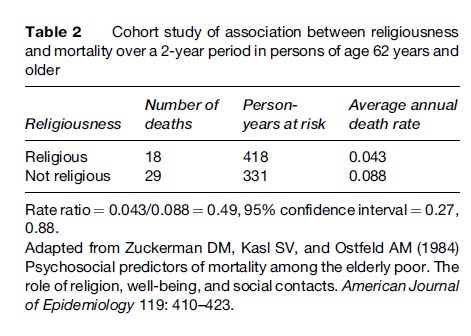
Table 2 shows results from a cohort study of whether religiousness is associated with a reduction in mortality rates in the elderly (Zuckerman et al., 1984). Mortality rates over the 2-year period of the study were in fact about 50% lower in the religious than in the nonreligious individuals. However, it is still debated whether religiousness itself is beneficial or whether some attribute associated with religiousness (e.g., a healthy lifestyle) is the reason for the lower death rate among religious people.

Cohort studies have a major advantage over case-control studies in that exposures or other characteristics of interest are measured before the disease has developed (or before changes in an attribute take place). On the other hand, cohort studies generally require large sample sizes, long-term follow-up of cohort members, large monetary expense, and complex administrative and organizational arrangements. The outcome of primary interest must be relatively common, or prohibitively large sample sizes will be needed to ensure adequate numbers experiencing the outcome. Therefore, prospective cohort studies are usually initiated under two circumstances: First, when sufficient (but not definitive) evidence has been obtained from less expensive studies to warrant more expensive cohort studies, and, second, when a new agent (e.g., a widely used medication) is introduced that may alter the risk for several diseases. In addition, cohort studies undertaken for one specific purpose are often used to test other hypotheses of interest as well.

Cohorts are sometimes chosen because they are representative of a certain community, such as in the Framingham Heart Study (Dawber et al., 1951), which started in 1948. This study is ongoing and now includes both offspring and grandchildren of the original cohort members. Although the ability to generalize from such studies makes them highly desirable, they are usually expensive and lose a substantial proportion of participants over the course of many years. Furthermore, an exposure of interest may be uncommon in the general population so that selection of a cohort with a higher proportion exposed may be more efficient. People working in a specific industry or occupation are commonly enrolled in cohort studies since (a) they often have exposures of particular interest, (b) are less likely to be lost to follow-up, (c) have a certain amount of relevant information recorded in their medical and employment records, and (d) in many instances undergo initial and then periodic medical examinations. Cohorts from health insurance plans also offer various advantages, including the records that are kept of all patient encounters with the health plan.

A cohort that has provided a great deal of information about risk factors for several diseases in women is the Nurses’ Health Study cohort. Nurses were selected not because of any particular occupational exposure, but because it was believed that their cooperation would be good and that they would report disease occurrence with a high degree of accuracy. The first nurses’ cohort was established in 1976 and included 121 700 nurses. Following such a large cohort over many years might be prohibitively expensive, except that most of the information is collected through a questionnaire sent through the mail. A cohort study of a second group of nurses was established in 1987.

Retrospective Cohort Studies

In a retrospective cohort study (also called an historical cohort study), investigators assemble a cohort by reviewing records to identify exposures in the past (often decades previously). Based on recorded past exposure histories, cohort members are divided into exposed and nonexposed groups, or according to level of exposure. The investigator then reconstructs their subsequent disease or mortality experience up to some defined point in time. For instance, cancer incidence during the period 1953–96 was determined in workers who had been employed for at least 6 months in three Norwegian silicon carbide smelters (Romundstad et al., 2001) and then compared to the cancer incidence in the population of Norway over the same time period. A greater number of lung cancer cases was found among the silicon workers than was expected on the basis of lung cancer rates in the general population.

Retrospective cohort studies have many of the advantages of prospective cohort studies, but can be completed in a much more timely fashion; consequently, they are considerably less expensive. However, only when the necessary information on past exposure has been recorded fairly accurately can a retrospective cohort study be undertaken with much likelihood of success. Tracing most of the cohort members must be possible in order to establish whether they developed the disease of interest (or have died). As with prospective cohort studies, a retrospective cohort study is usually feasible only when the outcome of interest is relatively common. Obtaining information on characteristics of the cohort members other than the exposure and outcome of primary interest is also frequently critical, so as to determine whether those with and without the exposure of interest are comparable in other relevant respects (e.g., smoking habits) and to allow statistical adjustment for differences. If such information is not available, interpretation of the study results may be ambiguous.

Cross-Sectional Studies

 In a cross-sectional, or prevalence, study, both the exposure to a hypothesized risk factor and the occurrence of a disease are measured at one time (or over a relatively short period of time) in a study population. Prevalence proportions (numbers of cases of existing disease per population at risk at a given point in time or short period of time) among those with and without the exposure or characteristic of interest are then compared. For a quantitative variable such as blood pressure, the distributions of the variables in the exposed and unexposed are compared.

Cross-sectional studies include all cases of a disease, new and old, at a given point or period in time. Thus, it is difficult to differentiate cause from effect. For instance, cross-sectional studies reporting higher proportions of smokers among persons with mental illnesses than among others (Lasser et al., 2000) are unable to determine whether smoking predisposes people to mental illness or whether people with mental illnesses tend to take up smoking. Interpretation of cross-sectional studies is generally clear only for attributes that do not change as a result of the disease, such as genotype. In addition, the cases with disease of long duration tend to be overrepresented, since such cases are more likely to be identified at a given point in time than cases who recover or die quickly. Accordingly, any association found between an exposure and a disease may be attributable to survivorship with the disease rather than to development of the disease.

Another use of cross-sectional studies is simply to describe the prevalence of a disease in a population. For such studies to be useful, the individuals studied should be representative of the population to whom the results are to be generalized. Patients seen in tertiary care centers or in the practice of any one physician are seldom representative of all persons in the community with a disease, many of whom may not have sought medical care. Generalizations from such select groups of patients should be avoided.

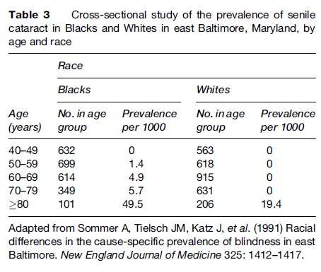
An example of a cross-sectional study with important public health implications is a study of the prevalence of causes of blindness in a sample of Blacks and Whites in east Baltimore, Maryland (Sommer et al., 1991). Whites were much more likely to have macular degeneration, and Blacks were more likely to have glaucoma. The prevalence of unoperated cataracts was high among middle-aged Blacks and among the elderly in both groups (Table 3). The authors suggest that about half of all blindness in this population is preventable or reversible and that certain population subgroups, such as Blacks and the elderly, should be targeted for education and intervention.

Hybrid Study Designs

Nested Case-Control Studies

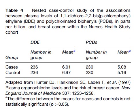
Sometimes it is possible to increase efficiency and maintain the advantages of a cohort study by designing a case control study within either a prospective or retrospective cohort study. Such a study is often referred to as a nested case-control study. Suppose blood samples from a cohort of 10 000 people free of rheumatoid arthritis at baseline have been frozen and stored. Suppose that after 10 years 200 people have developed rheumatoid arthritis and 9800 have not. The stored sera from the 200 people with rheumatoid arthritis and a sample of, say, 600 of the 9800 people free of rheumatoid arthritis are thawed and analyzed for the presence of some serologic marker. This sampling of nondiseased individuals greatly reduces the cost from what it would be in a traditional cohort study in which sera from all 10 000 cohort members would be tested at the beginning of the study. Nevertheless, the serologic marker was present before the disease developed, thus providing the major advantage of a cohort study. The serologic status of the cases and controls is then compared, as in a traditional case-control study. In a nested case-control study, controls are selected from unaffected cohort members who are still alive and under surveillance at the time the cases developed the disease. Typically, the controls are matched to cases according to age, sex, and time of entry into the cohort. The availability of many banks of stored serum around the world and the current interest in serologic predictors of disease make nested case-control studies an attractive and economical approach, as long as the serologic marker of interest does not undergo degradation over time. Similarly, genetic markers of disease can be examined in a nested case-control study, provided appropriate cells have been properly stored.

In a nested case-control study within the Nurses’ Health Study cohort (Hunter et al., 1997), plasma levels of organochlorine chemicals (mostly from pesticide exposure) were measured from the stored sera of nurses who developed breast cancer and a sample of nurses in whom breast cancer had not developed. Table 4 shows that cases did not have higher levels of either chemical than did controls.

Case-Cohort Studies

Another hybrid study design being used with increasing frequency is the case-cohort study. A case-cohort study is another method of increasing efficiency compared to a traditional retrospective or prospective cohort study and is particularly useful when the associations between a serologic marker (or other variable) and two or more diseases are of interest. As in a nested case-control study, all cases occurring in a cohort are generally selected for study. However, in a case-cohort study, the comparison group is a sample of the entire cohort, not just those free of disease, and the cohort members are not matched to the cases. Rather, other relevant variables and the possibility that some cases could be included in the comparison group are taken into account in the statistical analysis.

Cummings et al. (1998) used a case-cohort design within the Study of Osteoporotic Fractures, a prospective cohort study, to determine whether baseline concentrations of certain endogenous hormones predicted the occurrence of hip and vertebral fractures during follow-up. They compared hormone concentrations from stored serum samples of women who developed hip and vertebral fractures during follow-up with hormone concentrations from stored sera of a random sample of women from the same cohort. They found that undetectable serum estradiol concentrations and high concentrations of sex hormone-binding globulin at baseline were associated with increased risks for both hip and vertebral fractures.

Ecologic Studies

In an ecologic study, a summary measure of exposure and a summary measure of disease frequency are obtained for aggregates of individuals, such as persons in certain geographic areas or time periods. The purpose is to determine whether the units with the highest (or lowest) frequency of exposure tend to be the units with the highest (or lowest) frequency of disease. For instance, it has long been observed that countries with the highest per capita consumption of beer have the highest incidence rates of rectal cancer. However, there are many other differences among these countries in addition to their beer consumption. Additional analytic studies are needed to determine whether within these countries the individuals who drink the most beer have the highest rectal cancer rates. An ecologic study in the United States (McGwin et al., 2004) reported that states with lower mortality rates from motorcycle accidents were more likely than other states to require a skill test for a motorcycle permit, driver training, a long duration of a learner’s permit, three or more learner permit restrictions (e.g., no passengers, no riding at night), and a helmet for motorcycle operators of all ages. This report needs to be followed up by studies to determine whether individuals with these training characteristics are the ones with lower risk of death from motorcycle accidents, taking into account other relevant attributes such as the alcohol consumption of the individuals and the overall safety of the roads in the states.

When appropriate aggregated and individual-level data are available, two or more different levels of aggregation (e.g., state, county, municipality, census tract, block group, block, individual) can be considered in the same study and nested within each other to form a hierarchy of levels, each of which could be contributing to risk for the disease under study. Special methods of statistical analysis, called multilevel analysis or multilevel modeling, are used to try to separate out the contributions of the different levels of aggregation to disease risk.

Selected Epidemiologic Concepts In Observational Studies

Confounding

The possibility of confounding, which is especially likely to occur in observational studies, usually needs to be considered when trying to interpret associations between exposures and diseases. A confounding variable is a variable that (a) alters the risk of the disease or condition under study independent of the exposure or characteristic of primary interest, and (b) is associated with the exposure or characteristic of primary interest in the study population, but (c) is not a consequence of that exposure. Suppose that an investigator finds that coffee drinking during pregnancy is associated with an increased risk for delivery of a low-birth-weight infant. The investigator would have to be concerned that this statistical association between coffee consumption and delivery of a low-birth-weight infant is actually attributable to a tendency of coffee drinkers to smoke cigarettes to a greater extent than non-coffee drinkers, and that it is the cigarette smoking that puts them at an elevated risk for delivering a low-birth-weight infant, not the coffee drinking. In this instance, smoking is considered a confounding variable.

With any study design, information on potential confounding variables can be obtained during data collection and then controlled for in the statistical analysis. Alternatively, in cohort studies, one or more potential confounding variables may be taken into account in the study design by matching unexposed to exposed individuals on the potential confounding variable(s), which then must be taken into account in the statistical analysis by using stratification or regression methods. In case-control studies, controls may be matched to cases on one or more potential confounding variables, and the matching again taken into account in the analysis. It is possible to match roughly on certain variables in the study design and then control more tightly in the analysis. Measurement of potential confounding variables is highly important, because otherwise they cannot be adequately taken into account in the study design or analysis.

Effect Modification

Effect modification, also called statistical interaction, occurs when the magnitude of the association between one variable and another differs according to the level of a third variable. For instance, the association between obesity and risk for breast cancer varies according to whether a woman is premenopausal or postmenopausal. Among postmenopausal women, obese women are at elevated risk for breast cancer, while before menopause, obese women are not at increased risk for breast cancer and may even be at decreased risk compared to thin women. An area of considerable current interest is whether the effects on disease risk of certain environmental exposures and lifestyle factors are modified by a person’s genotype. For example, Hines et al. (2001) found that moderate alcohol drinkers as a group were at decreased risk for myocardial infarction compared to non-drinkers. However, an individual’s alcohol dehydrogenase type 3 (ADH3) genotype modified this association. Moderate alcohol drinkers who were homozygous for the slow-oxidizing ADH3 allele had greater high-density lipoprotein levels and a substantially decreased risk for myocardial infarction compared to moderate alcohol drinkers of other genotypes. In the statistical analysis, identification of effect modification involves comparing associations between exposures and diseases in subgroups of the population (e.g., in premenopausal vs. postmenopausal women; in those homozygous for the slow-oxidizing ADH3 allele vs. those of other genotypes).

Some Measures Of Association And Their Attributes

Relative Risk

In cohort studies, the strength of the association between a putative risk factor and a disease is often measured by what is called a relative risk (or more accurately, a rate ratio or risk ratio; a discussion of rate ratios and risk ratios is beyond the scope of this research paper). A relative risk is simply the risk (or incidence rate) of disease in one group (usually the exposed) divided by the risk (or incidence rate) of disease in another group (usually the unexposed). A relative risk (or, technically, a rate ratio) of 0.043/ 0.088 = 0.49 can be computed from Table 2, consistent with a beneficial effect of religiousness. Before reaching any conclusions, however, one would want to check for confounding by a variety of variables that are associated with religiousness and life expectancy, such as smoking habits, alcohol consumption, and many other attributes.

Odds Ratio

In case-control studies, risks and incidence rates usually cannot be determined because the investigator has selected the study population based on the presence or absence of disease and does not know disease frequency specifically in the exposed and unexposed. Therefore, relative risks cannot be computed. Rather, the odds ratio is calculated. In an unmatched case-control study, the odds ratio is estimated by the ratio of exposed to unexposed among cases divided by the ratio of exposed to unexposed among controls. In a case-control study in which controls are individually matched to cases, the odds ratio is estimated as the ratio of the number of case control pairs in which the case is exposed and not the control to the number of pairs in which the control is exposed and not the case. It can be shown that for all but the most common diseases (i.e., more than 10% of the exposed or unexposed population affected), the odds ratio is a good approximation to the relative risk and can be interpreted in a similar manner. In the case-control study described above of the association between smoking and lung cancer (Table 1), the odds ratio of

indicates that the odds of lung cancer in smokers is more than nine times that in nonsmokers. The odds ratio in the study mentioned previously of the association between phytoestrogen consumption and breast cancer was 1.0 for the highest quartile of consumption versus the lowest quartile, suggesting no association, either negative or positive, between phytoestrogen consumption and breast cancer.

Standardized Ratios

The standardized mortality ratio (SMR) and the standardized incidence ratio (SIR) are generally used when disease rates in the cohort under study are being compared to disease rates in a reference population, such as the general population of the geographic area from which the cohort was selected. The SMR (or SIR) is the ratio of observed number of deaths (or incident cases) in the cohort to the number of deaths (or incident cases) that would be expected, for example, on the basis of age and gender-specific death (or incidence) rates in the general population. The SIR of 1.85 (74 observed cases/39.9 expected cases) for lung cancer incidence in male Norwegian silicon carbide smelter workers (Romundstad et al., 2001) indicates that there are almost twice as many lung cancer cases among the smelter workers as would be expected based on the age and time-period-specific incidence rates in the male population of Norway.

Confidence Interval

A confidence interval should be presented along with estimates of the relative risk, odds ratio, or other parameter in order to give a range of plausible values for the parameter being estimated. A 95% confidence interval of 1.46–2.75 around a point estimate of relative risk of 2.00, for instance, indicates that a relative risk of less than 1.46 or greater than 2.75 can be ruled out at the 95% confidence level, and that a statistical test of any relative risk outside the interval would yield a probability value less than 0.05.

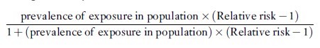
Attributable Fraction

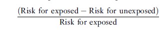
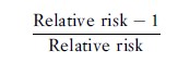
Provided that the association between a risk factor and a disease is causal (see the section titled ‘Guidelines for Assessing Causation from Observational Studies’ below), the attributable fraction provides a rough indication of the proportion of disease occurrence that potentially would be eliminated if exposure to the risk factor were prevented. It should not, however, be confused with the proportion of cases caused by the exposure or the probability of causation. The attributable fraction can be calculated either for exposed individuals only or for the population as a whole. In a cohort study, the attributable fraction for the exposed can be computed as

or, equivalently

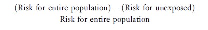
The attributable fraction for the population can be computed as

or, equivalently

In case-control studies of uncommon diseases, the odds ratio can be substituted for the relative risk to provide a good approximation to the attributable fraction that would be computed using the relative risk.

It is important to note that in the presence of confounding, other formulae must be used to estimate attributable fractions.

Measurement Error

Inaccurate measurement can lead to erroneous conclusions. The possibility of measurement error is of concern for most variables considered in observational epidemiologic studies. Exposures such as diet and physical activity are almost always measured by questionnaire, and their measurement can entail a great deal of error. Measurement of some diseases such as arthritic disorders and psychiatric disorders is difficult because of the frequent absence of definitive diagnostic criteria.

The validity or accuracy of a measurement refers to the average closeness of the measurement to the true value. Reliability or reproducibility refers to the extent to which the same value of the measurement is obtained on the same occasion by the same observer, on multiple occasions by the same observer, or by different observers on the same occasion. Precision refers to the amount of variation around the measurement or estimate; a precise measure will have a small amount of variation around it, but may or may not be valid. Measurement error is said to be differential if the magnitude of error for one variable differs according to the actual value of other variables, and nondifferential if the magnitude or error in one variable does not vary according to the actual value of other variables. In a 2 ×2 table (e.g., exposure present or absent, disease present or absent), nondifferential misclassification always causes the relative risk or odds ratio to be closer to 1.0 than the true value, provided that errors in measurement of the two variables are independent. Dependent, or differential, misclassification, on the other hand, can cause associations to be overestimated or underestimated, depending on the circumstances.

When measurement error occurs for a potential confounding variable, adjusting for the confounding variable in the analysis will not entirely remove its effect. When both the exposure and confounder are measured with error, effects are less predictable. Also, when estimates are made from tables larger than 2×2, there are circumstances under which even nondifferential measurement error can cause an association to appear larger than it really is.

Common Sources Of Bias In Observational Epidemiologic Studies

Bias refers to the tendency of a measurement or a statistic systematically to underestimate or overestimate the true value of that measurement or statistic. Bias can arise from many sources in observational epidemiologic studies. It can affect estimates of disease and exposure frequency and the magnitude of associations between exposures and diseases. Biases from uncontrolled confounding and from measurement error were described in previous sections. Some other common sources of bias are described in the following sections.

Information Bias

This is systematic error in measuring the exposure or outcome such that data are more accurate or more complete in one group than in another. Interviewer bias, recall bias, and reporting bias are examples of information bias.

Interviewer bias is systematic error occurring when an interviewer does not collect information in a similar manner for each group being compared. For example, if an interviewer believes, whether subconsciously or not, that a certain drug increases the risk for breast cancer, in a case-control study the interviewer might probe more deeply into the medication history of cases than controls.

Recall bias is systematic error resulting from differences in the accuracy or completeness of recall of past events between groups. In a case-control study, mothers of infants whose children are born with a congenital malformation may think back and remember events during the pregnancy more thoroughly than mothers of apparently healthy infants.

Reporting bias is a systematic error resulting from the tendency of people in one group to be more or less likely to report information than others. In a case-control study, cases with certain diseases might be more likely to deny that they had used alcohol than controls.

Selection Bias

This is systematic error occurring as a result of differences between those who are and those who are not selected for inclusion in a study or who are selected to be in a certain group within a study. Examples of selection bias are ascertainment bias, detection bias, and response bias.

Ascertainment bias is systematic error consequent to failure to identify equally all categories of individuals who are supposed to be represented in a group. For example, a specialty hospital may include mostly very sick or complicated cases who are not representative of all cases.

Detection bias is systematic error resulting from greater likelihood of some cases being identified, diagnosed, or verified than others. For instance, a diagnosis of pulmonary embolism may be more likely to be made in oral contraceptive users than in non-users because the oral contraceptive users may be more likely to have a lung scan for chest pain. As a result, an association between oral contraceptives and pulmonary embolism might result at least in part from greater likelihood of disease detection.

Response bias is systematic error resulting from differences between those who do and do not choose to participate in a study, and between those who remain in a cohort study and those who do not. In a study to estimate disease incidence or prevalence, even though a sample is scientifically selected, if a substantial proportion of those who are selected do not participate, the sample is likely to give biased results. In a study trying to estimate the prevalence of a disease, for instance, those with serious disease may be too sick to participate, and busy people may have little interest in participating. Accordingly, very ill and very busy people may be underrepresented in the study. If people who are sicker are less likely to return for follow-up visits in a cohort study, information on disease status of those who do continue to participate will not be representative of the disease status of all persons who were originally enrolled in the study.

Guidelines For Assessing Causation From Observational Studies

Because most epidemiologic studies are observational, conclusions about the likelihood of causation often have to be made on the basis of observational studies, despite their limitations and potential biases. In recent years, counterfactual, graphical, and structural equation models have begun to be applied to the analysis of possible causal relationships. Although beyond the scope of this research paper, these models are likely to see increasing applications in observational epidemiology in the future.

Over the years, epidemiologists have developed practical guidelines to be used as tests of whether a causal association exists. Not all criteria need to be fulfilled in all instances, nor are all equally important or always applicable. However, taken together, they provide some guidance about whether an association between a given exposure and disease is one of cause and effect.

• Strength of association: The measure of association (e.g., relative risk) should be elevated (or decreased for a protective factor), indicating that the exposed are at increased risk of disease compared to the unexposed. The higher the relative risk, the more likely the association is to be causal. As a rough rule of thumb, a relative risk or odds ratio of 2 suggests a moderate elevation in risk, and a relative risk of 3 or more is considered strong.
• Ruling out alternative explanations: Once it has been determined that an association between an exposure and disease exists, other explanations for the observed association, such as methodological deficiencies and confounding, should be carefully considered and tested against any available data or background information.
• Dose–response relationship: If increasing dose or length of exposure is associated with increasing risk, then the case for causality is considerably enhanced. The absence of a dose–response relationship, however, does not disprove causality since other patterns, such as a threshold effect, could also exist.
• Removal of exposure: If the presence of an exposure increases risk of disease and removing the exposure reduces risk, the likelihood of a causal association is increased.
• Time order: It should be clear that the exposure caused the disease and not that the disease caused the exposure. This issue is especially relevant in cross-sectional studies, in which prevalent cases and exposures are considered simultaneously. Time order is unique among the causal guidelines in that if the disease can be shown to have preceded the exposure, the exposure cannot have caused the disease.
• Predictive ability: Tentative hypotheses regarding causation that can be shown to predict future occurrences better than alternative hypotheses provide strong support for causality.
• Consistency: If associations of similar magnitude are found in different populations by different methods of study, the likelihood of causality is increased, since all studies are unlikely to have the same methodological limitations or idiosyncrasies of the study population.
• Biologic plausibility: When a new finding fits well with current knowledge of the biology of a disease, it is more plausible than if a whole new theory must be developed to explain the finding. Another way of enhancing biologic plausibility is through laboratory experiments. However, what occurs in a laboratory or in animals may have limited applicability to free-living humans.
• Coherence of evidence: The various relationships and findings should make biologic and epidemiologic sense.
• Confirmation in experimental studies: When available, the results of well-designed experiments in which exposures are assigned at random are very convincing because the only factor on which groups differ, except by chance, is the exposure of interest. However, in many circumstances, exposures cannot be ethically or practically assigned at random. In addition, experiments on carefully selected people may have limited relevance to the general, free-living population.

It should be apparent that decisions on the likelihood of causality are of necessity partly judgmental. What one person may believe is a causal association, another person may not. Lilienfeld (1957) divided the degree of evidence for causation into three levels (Table 5). At the first level, the evidence is considered sufficient for further study. For instance, studies suggesting that the risk of certain cancers is increased by high levels of exposure to electromagnetic fields fall into this category. At the second level, the evidence is considered sufficient to warrant public health action, even if the causal association has not been definitively established. Many people would put the evidence that a healthy diet protects against certain cancers at this second level. At the third level, the evidence is so strong that the causal association is considered part of the body of scientific knowledge. The evidence that smoking causes lung cancer or that the human immunodeficiency virus causes AIDS is at this level of certainty.

Conclusion

Observational epidemiology plays an important role in learning about disease causation. Major concerns of epidemiologists undertaking observational epidemiologic studies include using the best sources of data, employing the proper study designs, selecting appropriate study populations, using good methods of measurement, quantifying the magnitudes of associations, controlling for confounding, and detecting effect modification. In practice, it is often not possible to meet all these objectives to the extent desired because people may choose not to participate in a study, optimal measurement may not be feasible, and a variety of other problems may arise. It is important to recognize the effects of these inadequacies in various situations because specific inadequacies can affect study results in different ways.

It should be readily apparent that conclusions drawn from observational epidemiologic studies, as with other types of scientific inquiry, are often not final. Results generally require confirmation from additional epidemiologic or laboratory studies, experimental studies, or ascertainment of the effect of removal or modification of the suspected risk factor. What was believed to be a causal association may later be found to be attributable to uncontrolled confounding, and an association thought to be attributable to uncontrolled confounding may turn out to be causal. A causal agent in one population may not operate the same way in another population. The best method of measurement at one point in time may later be supplanted by a better method. In any one study, a reported association may have occurred by chance, especially when many possible associations are being examined.

Thus, it is essential to keep an open mind as new knowledge accumulates about disease causation from epidemiologic, laboratory, and other types of studies and as attempts are made to replicate the results of even the most carefully executed individual studies. In this way, knowledge about disease causation gradually evolves.

Bibliography:

1. Cummings SR, Browner WS, Bauer D, et al. (1998) Endogenous hormones and the risk of hip and vertebral fractures among older women. Study of Osteoporotic Fractures Research Group. New England Journal of Medicine 339: 733–738.
2. Dawber TR, Meadors GF, and Moore FE Jr (1951) Epidemiological approaches to heart disease: The Framingham Study. American Journal of Public Health 41: 279–286.
3. Doll R and Hill A (1952) A study of the aetiology of carcinoma of the lung. British Medical Journal 2: 1271–1286.
4. Dowell SF, Kupronis BA, Zell ER, et al. (2000) Mortality from pneumonia in children in the United States, 1939 through 1996. New England Journal of Medicine 342: 1399–1407.
5. Goh KJ, Tan CT, Chew NK, et al. (2000) Clinical features of Nipah virus encephalitis among pig farmers in Malaysia. New England Journal of Medicine 342: 1229–1235.
6. Hines LM, Stampfer MJ, Ma J, et al. (2001) Genetic variation in alcohol dehydrogenase and the beneficial effect of moderate alcohol consumption on myocardial infarction. New England Journal of Medicine 344: 549–555.
7. Horn-Ross PL, John EM, Lee M, et al. (2001) Phytoestrogen consumption and breast cancer risk in a multiethnic population: The Bay Area Breast Cancer Study. American Journal of Epidemiology 154: 434–441.
8. Hunter DJ, Hankinson SE, Laden F, et al. (1997) Plasma organochlorine levels and the risk of breast cancer. New England Journal of Medicine 337: 1253–1258.
9. Jacobus CH, Holick MF, Shao Q, et al. (1992) Hypervitaminosis D associated with drinking milk. New England Journal of Medicine 326: 1173–1177.
10. Lasser K, Boyd JW, Woolhandler S, et al. (2000) Smoking and mental illness: A population-based prevalence study. Journal of the American Medical Association 284: 2606–2610.
11. Lilienfeld A (1957) Epidemiologic methods and inferences in studies of non-infectious diseases. Public Health Reports 72: 51–60.
12. Maguire-Boston EK, Suman V, Jacobsen SJ, et al. (1999) Blood transfusion and risk of non-Hodgkin’s lymphoma. American Journal of Epidemiology 149: 1113–1118.
13. Mason TJ, McKay FW, Hoover R, et al. (1975) Atlas of Cancer Mortality for US Counties: 1950–1969 Washington, DC: US Department of Health Education, and Welfare. DHEW Publication No. (NIH) 75–750.
14. McGwin G Jr, Whately J, Metzger J, et al. (2004) The effect of state motorcycle licensing laws on motorcycle driver mortality rates. Journal of Trauma 56: 415–419.
15. Miettinen OS (1985) The ‘‘case-control’’ study: valid selection of subjects. Journal of Chronic Diseases 38: 543–548.
16. Romundstad P, Andersen A, and Haldorsen T (2001) Cancer incidence among workers in the Norwegian silicon carbide industry. American Journal of Epidemiology 153: 978–986.
17. Sommer A, Tielsch JM, Katz J, et al. (1991) Racial differences in the cause-specific prevalence of blindness in east Baltimore. New England Journal of Medicine 325: 1412–1417.
18. Zuckerman DM, Kasl SV, and Ostfeld AM (1984) Psychosocial predictors of mortality among the elderly poor. The role of religion, well-being, and social contacts. American Journal of Epidemiology 119: 410–423.
19. Austin H, Hill HA, Flanders WD, et al. (1994) Limitations in the application of case-control methodology. Epidemiologic Reviews 16: 65–76.
20. Friedman GD (2004) Primer of Epidemiology, 5th edn. New York: McGraw-Hill Inc.
21. Gordis L (2000) Epidemiology, 2nd edn. Philadelphia, PA: WB Saunders Company.
22. Greenland S (2000) Causal analysis in the health sciences. Journal of the American Statistical Association 95: 286–289.
23. Greenland S (2001) Ecologic versus individual-level sources of bias in ecologic estimates of contextual health effects. International Journal of Epidemiology 30: 1343–1350.
24. Kelsey JL, Whittemore AS, Evans AS, et al. (1996) Methods in Observational Epidemiology, 2nd edn. New York: Oxford University Press.
25. Koepsell TD and Weiss NS (2003) Epidemiologic Methods. Studying the Occurrence of Illness. New York: Oxford University Press.
26. Last JM (ed.) (2001) A Dictionary of Epidemiology, 4th edn. New York: Oxford University Press.
27. Rothman KJ and Greenland S (1998) Modern Epidemiology, 2nd edn. Philadelphia, PA: Lippincott Raven.
28. Szklo M and Nieto FJ (2000) Epidemiology, Beyond the Basics. Gaithersburg, MD: Aspen Publishers.

See also:

• How to Write a Research Paper
• Research Paper Topics
• Research Paper Examples

Free research papers are not written to satisfy your specific instructions. You can use our professional writing services to buy a custom research paper on any topic and get your high quality paper at affordable price.