
This sample Philosophy of Forensic Identification Research Paper is published for educational and informational purposes only. If you need help writing your assignment, please use our research paper writing service and buy a paper on any topic at affordable price. Also check our tips on how to write a research paper, see the lists of criminal justice research paper topics, and browse research paper examples.
In most if not all criminal investigations, the collection, examination, and interpretation of physical evidence plays a major role. Material traces, whether they are of a physical, chemical, biological, or digital nature, may serve to suggest or support plausible scenarios of what might have happened at a possible scene of crime. Ultimately, they may be instrumental in distinguishing between the rival scenarios that the judge or jury will have to consider in arriving at the final verdict: Was the crime committed by the suspect in the way described by the prosecution, was it someone else who did it, or was no crime committed in the first place?
Individualization of physical traces, like DNA, handwriting, or fingerprints, logically amounts to a process of inference of identity of source between a crime scene trace and some reference material whose origin is known. While its aim is to uniquely identify the source of the trace and many criminalists, most notably the dactyloscopists, have long proceeded as though individualization of traces is a routine affair, there is no scientific basis for this claim or for the methods by which individualization or source attribution is supposedly achieved. It is largely as a result of the advent of forensic DNA analysis and the conceptual framework associated with the interpretation of DNA evidence that the forensic community has come to appreciate the “individualization fallacy” (Saks and Koehler 2008) and the consequent need to adopt what has come to be known as a logical or Bayesian approach to the interpretation of technical and scientific evidence.
A comprehensive model for the assessment and interpretation of forensic evidence along Bayesian lines was developed in Britain by Ian Evett and colleagues at the Forensic Science Service (Cook et al. 1998a, b; AoFSP 2009; Evett 2011). It defines a hierarchy of propositions to be addressed in casework which is composed of three levels and extends over two domains. The first domain, that of the forensic expert, involves propositions at the level of source and at the level of activity. Propositions at the level of source address the question of the origin of the trace, while propositions at the activity level relate to the question how and when the trace arose. Propositions formulated at the third level, termed the level of offense, belong exclusively to the domain of the trier of fact and relate to the ultimate, legal issue whether an offense was committed and if so, whether it was committed by the defendant.
While the Bayesian approach provides an excellent framework for the evaluation and interpretation of expert evidence in that it helps define the relevant questions and draws a sharp line between the domain of the expert and that of the trier of fact, it is not an intuitively easy approach. A clear and transparent exposition of the method used by the expert to determine the weight of the scientific evidence is therefore of the essence. Recent research as well as court decisions suggest that if this information is lacking judges and juries will be hard put to assess the evidence at its true value.
Criminalistic Processes: Individualization Versus Identification
In order for material traces like DNA to be able to contribute to criminal investigations in the form of technical or scientific expert evidence, there are various questions that need to be addressed. One question seeks to determine the nature or substance of the trace material. Are we dealing with blood, gunshot residue, MDMA, or hair? The process by which this type of question is answered is called identification.
A second process, classification, takes the first process one step further. It is undertaken to determine whether the crime scene trace can be assigned to a particular group or class of similar objects or substances. Examples of classification processes in the forensic sciences are: the classification of blood into human versus animal blood; of hair into animal versus human hair and, beyond that, the (sub)classification into body, head, and pubic hair; the classification of fibers into man-made versus natural fibers; the classification of firearms and cartridges in terms of their make and caliber, or that of shoes according to size, make, model, sole pattern, etc.
A third process seeks to identify the origin or source of the trace material. Is it possible to relate the trace or the carrier of the trace to a particular person or object? This process, the determination of the unique source of a trace, is technically called individualization and is often seen as the process that lies at the heart of the criminalistic effort. Although, in common parlance, the term “identification” may also be used for the process of source determination, as in a phrase like fingerprint identification or indeed in the title of this research paper, the proper technical term for this process is individualization.
A fourth question concerns the relation of the trace material with the crime by trying to establish how and when the trace was generated. This process, which focuses on the nature of the activity by which the trace material arose, is often referred to as association.
All four processes, identification, classification, individualization, and association, are essential elements of the larger process of reconstruction (Inman and Rudin 2000): the attempt to create coherent scenarios of the chain of events that constitutes the incident under examination on the basis of the available evidence.
Particularly in the context of DNA evidence, both “source level” questions of the type “Whose DNA is it?” and “activity level” questions of the type “How and when did the cell material get there?” are of paramount importance, as it is only on the strength of the combined answers to these questions that a link can be established between a particular person or object and a possible crime.
Conclusions in Individualization Criminalistics is the science of individualization (Kirk 1963, p. 235)
Individualization may be defined as the process undertaken to establish the unique source or origin of a particular material trace. Put simply, it tries to answer questions like “Whose DNA/handwriting/ fingerprint, etc. is this?” According to Paul Kirk (1902–1970), one of the founding fathers of criminalistics, it is individualization that marks off criminalistics as a science from other sciences.
While the goal of criminalistics is always the same, there are considerable differences in the methodology used and the conclusions formulated by the practitioners of the various forensic disciplines to achieve this aim. By and large, three groups may be distinguished in terms of the way in which the conclusions of a comparative trace examination are expressed. First, the conclusions may directly address the probability of the source hypothesis given the evidence. This tends to be the case in dactyloscopy and typically also still holds for most other types of source level trace examinations. An important exception is DNA, where the conclusions expressed relate to the probability of the evidence under a particular hypothesis rather than to the probability of the hypothesis given the evidence. Second, unlike dactyloscopists, who will generally express their conclusions in categorical terms, forensic experts in most other fields of trace examination will tend to express their conclusions in probabilistic terms, in either a verbal format or in a quantitative format, as in DNA typing.
Schematically, where C stands for categorical, P for probabilistic, E for statement of the probability of the evidence, and H for statement of the probability of the hypothesis, the following distinctions may be noted:
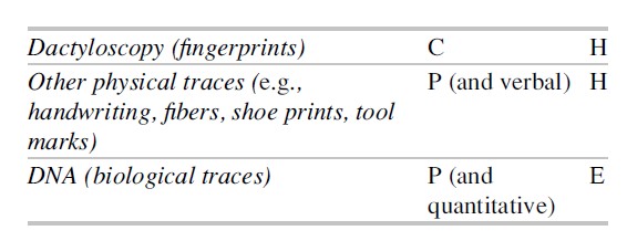
For example, the dactyloscopist will conclude that a finger mark does or does not originate from a particular (person’s) finger, thereby making a categorical statement of the probability of H, the source attribution hypothesis. But the handwriting expert will – traditionally anyway – typically conclude that the questioned writing probably/very probably/with a probability bordering on certainty does – or does not, as the case may be – originate from the writer of the reference material, thereby making a (verbal) probabilistic rather than a categorical statement of H, the source hypothesis.
By contrast, the DNA expert will first determine whether the source material could originate from the person whose reference profile is being compared with that of the crime scene sample. If the profiles of the crime scene material and the person under investigation match, the expert will state that the crime scene material may originate from this person. To indicate the significance of this finding, the expert will add how likely the evidence, i.e., a matching profile, is if the crime scene material originates from the “matching” person under investigation as opposed to a random member of the population. Alternatively, the expert may report the estimated frequency of the profile in the relevant population. A third way to report the weight of the evidence is in terms of the so-called random match probability of the profile: The probability that a randomly chosen member of the population who is not related to the donor of the cell material or the matching suspect will match the crime scene profile.
It appears therefore that while the experts in the diverse fields are answering the same question, that of the origin of the trace, they will tend to use different conclusion formats to express their findings. The notions underlying these differences are explored below.
The Classical Approach To Individualization: The Underlying Principles
The traditional forensic approach to trace individualization is based on four – partly implicit – principles:
- The principle of transfer of evidence
- The principle of the divisibility of matter
- The uniqueness assumption
- The individualization principle
The Transfer Principle: “Every Contact Leaves A Trace”
The first of these, the transfer principle, is captured in the phrase “Every contact leaves a trace.” It expresses the notion that in the commission of criminal acts, invariably some traces will be left on the scene. It provides a theoretical basis for the generation of traces and a principled argument for the examination of the crime scene for traces. This insight was formulated most clearly by the Frenchman Edmond Locard (1877–1966), who was the first director of the Laboratoire de Police Scientifique in Lyon, France, in 1912 and is universally acclaimed as one of the fathers of criminalistics. While Locard was primarily thinking of the transfer of microscopic traces like dust, dirt, nail debris, or fibers, as left in the commission of the more violent type of crime, Locard’s exchange principle, as the principle is also commonly referred to, is also applicable to traces that arise in the context of less violent crimes as well as to latent (hidden), patent (visible to the naked eye), or plastic impression evidence, such as finger marks, tool marks, footwear marks, or striation marks on bullets and cartridge cases. In the latter case, it is not so much the physical matter that is deposited at or taken away from the crime scene that is of interest but the patterns or shapes that are transferred from donor (object) to recipient (object). In addition, the principle increasingly applies to so-called contact traces, as in DNA evidence. Here, terms like “trace DNA” or “touch DNA” are used to refer to cell material and debris transferred through skin contact, which may arise as a result of regular use, as on a watch, from a single, firm contact, as on a tie wrap or strangulation cord, or from a single touch, as on a glass surface (Raymond et al. 2004).
As Locard observed at the time, transfer may go either way. Traces like glass fragments, blood stains, hairs, or fibers are left at the crime scene by a donor and may be picked up from there by a receptor. If (part of) the material collected is subsequently left by the receptor and picked up by a second receptor, we speak of secondary transfer. For example, fibers or DNA material picked up by A from B’s clothing may be transferred from B’s clothing to chair C, and eventually end up on the clothing of D. In principle, forms of tertiary and quarternary transfer might also occur.
The Divisibility Of Matter: “Matter Divides Under Pressure”
The second underlying principle of criminalistics, that of the divisibility of matter, was explicitly defined only relatively recently by the American DNA experts Keith Inman and Norah Rudin (2000). It explains why transfer can play such an important role in the generation of traces. Although the principle as such is fairly obvious, it is of considerable importance for a proper understanding of the relation between the way traces arise and their interpretation. In an article entitled “The origin of evidence,” Inman and Rudin (2002: p. 12) describe the process of the division of matter and its results as follows:
Matter divides into smaller component parts when sufficient force is applied. The component parts will acquire characteristics created by the process of division itself and retain physico-chemical properties of the larger piece
This mechanism has important implications for the relation between traces and their sources. They are:
Corollary 1 Some characteristics retained by the smaller pieces are unique to the original item or to the division process. These traits are useful for individualizing all pieces to the original item.
Corollary 2 Some characteristics retained by the smaller pieces are common to the original as well as to other items of similar manufacture. We rely on these traits to classify them.
Corollary 3 Some characteristics from the original item will be lost or changed during or after the moment of division and subsequent dispersal; this confounds the attempt to infer a common source. (Inman and Rudin 2002, p. 12)
While the two principles discussed so far relate to the creation or generation of traces, the following two principles are central to the interpretation of traces, as viewed in the traditional approach to trace individualization.
The Uniqueness Assumption: “Nature Never Repeats Itself”
The first of these is the uniqueness assumption. It is nicely captured in the phrase “Nature never repeats itself” and essentially simply states that no two objects are identical. Or, as Kirk and Grunbaum (1968, p. 289) put it:
Now most students believe that all items of the universe are in some respect different from other similar items, so that ultimately it may be possible to individualize not only a person but any object of interest. This effort is the heart of criminalistics.
The uniqueness assumption was probably most vigorously championed by the fingerprint fraternity. However, before the fingerprint was discovered as a means to verify a person’s identity and subsequently came to be used for forensic purposes, the same principle provided a basis for forensic anthropometry, which was developed by the Frenchman Alphonse Bertillon (1853–1914).
Anthropometry. Anthropometry was developed by Bertillon primarily to identify repeated offenders. The method is based on an assumption derived from the Belgian astronomer and statistician Adolphe Quetelet (1796–1874) that no two human bodies are equal. A founder of modern quantitative sociology, Quetelet is not only believed to be the inspiration for the frequently cited phrase that nature does not repeat itself but must also be credited with the definition of the Quetelet index, which, since 1972, has come to be more widely known as the BMI or Body Mass Index.
The anthropometric method consisted in recording the dimensions of an arrestee’s body in terms of seven and later 12 measurements of a fixed set of parts of the body, including total physical height, the length and width of the head, the right ear, and the left foot, which were believed to be constant for adult members of the human race. In 1883, Bertillon succeeded in identifying a repeated offender by comparing his measurements with anthropometric data recorded earlier. Later in his life, Bertillon was the first to make a fingerprint identification in a murder case on the European Continent (Thorwald 1965, p. 83).
The assumption of uniqueness, together with the temporal stability of fingerprints, or friction ridge patterns as they are more technically called, is often adduced as a theoretical ground for the justification of the use of categorical conclusions of origin, as has typically been common if not universal practice in dactyloscopy. However, as Saks and Koehler (2005, p. 892) put it, in formulating these categorical conclusions, dactyloscopists in fact rely on a flawed notion of “discernible uniqueness.” The real issue in source attribution is not whether all possible sources can be distinguished from each other in principle, which is what the uniqueness assumption – presumably correctly – implies. The crucial question is whether a trace, which, due to the factors described under the divisibility principle, will inevitably differ to some extent from its particular source, can be attributed – with certainty, or, failing that, with any reliable degree of probability – to that source.
The Individualization Principle: “That Can’t Be A Coincidence”
The fourth principle in the traditional approach to trace individualization states that a conclusion of (probable) common origin of a trace and reference material – as in a comparative examination of a questioned handwriting sample and a reference sample from a known person – may be arrived at if there are so many similarities of such significance that their occurring together by chance may be practically excluded. As the American handwriting expert R.A. Huber (1959–1960, p. 289) put it in his definition of what he called “the principle of identification”:
When any two items have characteristics in common of such number and significance as to preclude their simultaneous occurrence by chance, and there are no inexplicable differences, then it may be concluded that they are the same, or from the same source.
The suggestion here is that a criterion, i.e., “of such number and significance,” may be defined which will provide a principled and objective way to determine that the possibility (or probability) that two objects meet this criterion by chance can be excluded. Such a criterion is not only not feasible in practice, as it begs the question what number and what degree of significance is required, but it also lacks a theoretical basis in that it ignores the essentially inductive nature of the individualization process.
The reason why individualization is problematic from a theoretical point of view is that any attempt to identify the unique source of physical, biological, or pattern evidence like finger marks, footwear marks, DNA, or handwriting is typically frustrated by the induction problem. We cannot, solely on the strength of even an extreme degree of similarity between trace and reference material, conclude that a particular trace must have originated from some specific reference material to the exclusion of all other possible sources, unless we have been able to examine all these alternative sources and eliminate them categorically.
To begin with, the population from which a finger mark or a questioned handwritten text actually originates is typically indefinite in size and frequently largely unavailable for examination. But even if it were possible to examine a large number of potential writers or fingers, we could not exclude finding one or more whose reference handwriting or fingerprint would show a similar or even greater degree of similarity with the questioned handwriting or finger mark than did the reference sample of the suspect. Since this possibility cannot be excluded, the individualization problem tends to be impossible to solve and in that sense is strongly reminiscent of that of Popper’s white swans: We cannot conclude that all swans are white unless we have been able to examine all swans (Popper 1959). Nor for that matter can we conclude that the trace probably originates from the reference material with which it shares many features. Indeed, although the observed degree of similarity between trace and possible source will tend to make the hypothesis of identity of source more probable in relative terms than it was before the comparative examination was carried out, similarity is neither a sufficient nor even a necessary condition for identity of source in absolute terms.
It is interesting that the individualization criterion as captured in the phrase “That cannot be a coincidence” is essentially similar to that used in traditional, standard textbook statistical significance testing. In this approach, the result of a hypothesis test is termed significant if it is unlikely to have occurred by chance. More specifically, the so-called null hypothesis that the result is due to chance may be rejected if the obtained result is less likely to occur under this hypothesis than a predetermined threshold probability of – frequently – 1 or 5 %. Like the traditional identification paradigm, this approach is also coming in for more and more criticism, partly because it also fails to take account of the probability of the result under the alternative hypothesis.
Class Characteristics Versus Individual Characteristics
In an attempt to overcome the induction problem traditional forensic identification, experts frequently rely on the distinction between class characteristics and individual characteristics. For example, all firearms of a particular make and caliber may leave the same markers on a cartridge or bullet, thereby making it possible to identify the type of weapon on the basis of the class or system characteristics that the particular type of firearm is known to leave. However, a certain configuration of striation marks left on a bullet may be distinctive for a particular weapon. As Thornton and Peterson (2002) put it:
Class characteristics are general characteristics that separate a group of objects from a universe of diverse objects. In a comparison process, class characteristics serve the very useful purpose of screening a large number of items by eliminating from consideration those items that do not share the characteristics common to all the members of that group. Class characteristics do not, and cannot establish uniqueness.
Individual characteristics, on the other hand, are those exceptional characteristics that may establish the uniqueness of an object. It should be recognized that an individual characteristic, taken in isolation, might not in itself be unique. The uniqueness of an object may be established by an ensemble of individual characteristics. A scratch on the surface of a bullet, for example, is not a unique event; it is the arrangement of the scratches on the bullet that mark it as unique.
Unfortunately, the definition of individual characteristics is circular. They are defined as characteristics that are – collectively – capable of establishing uniqueness. But whether an ensemble of individual characteristics is unique is itself an inductive question: We can never be sure that a feature or combination of features is unique, until we have observed all relevant objects, which is impossible.
What practitioners of traditional forensic identification sciences really do is perhaps best described by Stoney (1991), who used the image of the “leap of faith” as the mechanism whereby the forensic scientist actually establishes individualization, as in dactyloscopy:

When more and more corresponding features are found between the two patterns scientist and lay person alike become subjectively certain that the patterns could not possibly be duplicated by chance. What has happened here is somewhat analogous to a leap of faith. It is a jump, an extrapolation, based on the observation of highly variable traits among a few characteristics, and then considering the case of many characteristics… In fingerprint work, we become subjectively convinced of identity; we do not prove it.
Ultimately then, in traditional identification disciplines, in reaching a conclusion about the probable or categorical origin of the trace material, the expert delivers an essentially subjective opinion. When informed by adequate levels of training, experience, and expertise, this conclusion will frequently be correct, but it must be clear that the expert becomes convinced of the (probable) origin of the trace. He does not “prove” it: There is no logical basis for the conclusion.
The Logical Approach To Individualization: The Concept Of The Likelihood Ratio
By contrast, in the logical approach, the expert does not primarily seek to determine the probability of the source or activity hypothesis. Instead, the purpose of the comparative examination is to determine the likelihood of the evidence under two mutually exclusive propositions or hypotheses. Suppose we find a size 14 shoeprint at a crime scene and a suspect emerges who takes size 14. It will be clear that the shoe size information by itself gives us insufficient basis to say that it was the suspect who left the print rather than one of the other shoe size 14 wearers in the area (or beyond). The mere fact that the suspect wears size 14 shoes does not make him more suspect than anybody else with this size shoes. At the same time, it is clear that the finding looks incriminating. Or is it a mere coincidence?
The likelihood ratio (LR) provides a principled way to address this question. To calculate it, we need to determine the ratio of the likelihood of a size 14 turning up at the crime scene under two rival hypotheses: (1) The shoe mark was left by the suspect versus (2) the mark was left by a random member of the relevant potential donor population. We know that the likelihood of finding a size 14 mark if the suspect left it (and assuming he does not occasionally or otherwise wear a different size shoe) is 1, or 100%. To assess the likelihood of finding a size 14 shoe mark under the alternative hypothesis that a random member of the relevant population left the print, we need to know what percentage of that population takes a size 14 shoe. Suppose we know this figure to be 4 %. We can now calculate the likelihood ratio of the evidence under these two competing hypotheses, which in this case would amount to 100/4 = 25.
We can paraphrase this result by saying that the footwear evidence is 25 times more likely if the suspect left the mark than if a random member of the population left it. We can also say that the evidence makes it (25 times) more likely that the suspect left the mark than we believed was the case before we obtained the evidence. But we cannot on the basis of the shoe mark evidence alone pronounce upon the probability of the hypothesis that the suspect left the mark in absolute terms. Alternatively, what we can say in a case like this is that an LR of 25 reduces the group of potential suspects by a factor 25, leaving just one potential suspect on average for every 25 potential suspects considered before the shoe print evidence became available.
Similarly, when applied to DNA evidence, the likelihood ratio is a measure of the weight of the evidence and may be seen as an indication of the extent to which the uncertainty about the source hypothesis is reduced by the evidence. If, for example, the matching profile is known to have a frequency of 1 in a million in the relevant population, the LR of the matching DNA evidence may be reported as one million: It is the ratio of the likelihood of the evidence under the hypothesis that the person under investigation is the donor of the DNA material, i.e., 1 (or 100 %) divided by the likelihood of the evidence under the alternative hypothesis that the DNA originates from a random member of the population, i.e., 1/1,000,000. The conclusion implies that the evidence is a million times more likely if the crime scene sample originates from the donor of the reference material than if a random member of the population were the donor of the crime scene sample. It is only if there is no match that the DNA expert may make a – negative – categorical statement of the probability of the hypothesis.
Discrete Versus Continuous Variables
In the examples involving DNA and shoe sizes discussed above, the variables of interest are discrete or categorical in nature and the similarity between trace and reference material could be said to be either complete or to be entirely absent: The DNA profiles and the shoe sizes are the same or they are different. If they are different, the suspect’s shoe or body can be eliminated as the source of the trace. However, in many cases, the correspondence between trace and source will not be perfect. Many variables are not discrete (like DNA markers or shoe size) but continuous. Examples are quantitative variables such as length, weight, or shape. For these variables, there will always be a difference between trace and reference materials because in both cases, we are dealing with samples that will at best only approximate the “true,” i.e., average, population value for the feature of interest.
Again, handwriting analysis may serve as a case in point, but the same holds for any other type of trace with continuous properties like tool marks, fibers, speech, glass, or paint. Both the questioned writing and the reference writing must be seen as samples taken from the indefinitely large population of handwriting productions that the writers of these samples are capable of producing. This means that any marker that is examined, like the shape and execution of the letter t or the figure 8, will exhibit a certain degree of variability even within samples originating from the same source. However, traces originating from a single source will typically show a relatively small degree of within-source variation, while samples of material originating from different sources will typically show a relatively larger degree of between-source variation. As a result, in these cases, the numerator of the likelihood ratio will not be 100 % or 1, but say 80: A degree of similarity as great as that found between trace material and reference material will then be found in 80 % of cases if both originate from the same source and in say only 10 % of cases if trace material and reference material originate from different sources. The likelihood ratio would then be 80/10 = 8.
If, however, the degree of similarity found would be expected in only 20 % of cases under the hypothesis of common origin and in 40 % of cases under the hypothesis of different origin, the likelihood ratio would be 20/40 = ½, and the evidence would actually weaken the common source hypothesis rather than strengthen it. In the first instance, the likelihood ratio would exceed 1 and the evidence would (weakly) support the hypothesis of common origin; in the second instance, the likelihood ratio would be less than 1 and the evidence would – again weakly – support the alternative hypothesis, that the trace did not originate from the same source as the reference material.
The Likelihood Ratio And The Diagnostic Value
The concept of the likelihood ratio is similar to that of the diagnostic value, a measure which has found wide acceptance in fields like medicine and psychology as a way to express the value of a diagnostic test result. It is arrived at by dividing the relative number of correct (positive or negative) results of the test in question by the relative number of false (positive or negative) results of the test. In more technical language, by dividing the sensitivity of the test by (1 – the specificity). The sensitivity of the test is the percentage of correct positives it produces, the specificity the percentage of correct negatives. Applied to an HIV test, if the sensitivity of the test is 98 % and the specificity is 93 %, this would mean that 98 % of those infected would (correctly) test positive and 7 % of those not-infected would (incorrectly) also test positive. The diagnostic value of a positive result for the test would then be 98/(100-93) = 14 and the probability of the patient being infected would be 14 times greater now that the test result is known than whatever it was estimated to be before the test result was known. The diagnostic value of a negative test result would in this case be 93 (the relative number of correct negatives) divided by (100-98) = 2, the relative number of false negatives, i.e., 93 divided by 2 or 46.5.
Scientific evidence may be said to have diagnostic value in much the same way as a medical test such as an HIV test, which will not provide absolute proof of infection or otherwise but, depending on the result and its diagnostic value, will make infection more or less probable. Similarly, evidence may be more or less likely under one of two rival hypotheses. To the extent that the evidence favors, or better fits one hypothesis rather than another, it may be said to lend more support to that hypothesis.
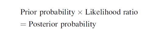
Bayes And The Prior Probability
The likelihood ratio may be seen as a measure of the extent to which the hypothesis of interest is more probable or less probable after the scientific evidence is known than it was before the evidence was known. Another way of putting it is to say that we can update what we saw as the prior probability of the hypothesis with the evidence that has become available to arrive at the posterior probability of the hypothesis, in which the weight of the new evidence has been taken into account. By means of the Bayes’ Rule, the odds form of Bayes’ theorem, so called after the Rev. Thomas Bayes (1702–1761), we can calculate the posterior probability of a hypothesis by multiplying its prior probability with the likelihood ratio:
A simple example may illustrate the application of the rule. Suppose a prisoner is found dead and we may safely assume that one of the 99 remaining fellow prisoners in the ward is the perpetrator. As it happens, one of these 99 prisoners, S, admits to being the killer. His DNA profile is obtained and found to match with a partial profile obtained from the nail debris secured from the victim. The estimated frequency of the partial profile in the relevant population is 1 in 1,000.
If the cell material in the nail debris originates from S, the likelihood of the evidence, i.e., the matching profile, would be 1, or 100 %. If, on the other hand, the cell material belonged to a random member of the population, the likelihood of a match would be 1 in 1,000 or 0.001. The likelihood ratio of the DNA evidence would therefore be 1 divided by 0.001 = 1,000.
To determine the prior probability, we assume that all 99 remaining prisoners are equally likely to be the perpetrator. In that case, the prior probability of any one of them being the donor is 1/99, or, expressed in odds, 1 to 98. We can now calculate the prior probability of S being the donor of the cell material in the nail debris by applying Bayes’ rule:
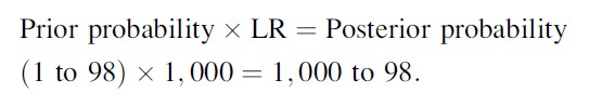
The odds form of the posterior probability may be converted to a fraction, i.e., 1,000/1,098, and from that into a percentage, i.e., 91.1 %. This means that on the basis of the DNA evidence alone, the probability of the suspect being the donor of the cell material is 91.1 %, assuming that the donor is one of the remaining 99 prisoners.
Of course, apart from the DNA evidence, the fact that S admitted to killing his fellow inmate is also relevant to the determination of the ultimate issue whether S is the perpetrator. However, this type of evidence as well as possible eyewitness accounts from fellow prisoners or prison staff, and any other non-DNA evidence, clearly extends beyond the domain of the DNA expert. Other experts might be able to assign a particular weight to a spontaneous confession or an eyewitness identification, in the form of a likelihood ratio. For example, empirical research may be available on which an estimate may be based of the diagnostic value (= likelihood ratio) of a confession. This could take the form of a statement that a confession is on average seven times more likely if the suspect is the perpetrator than if he is not. This evidence in turn could then be used to further update the hypothesis of guilt.
When Numbers Are Lacking
It is worth noting that the concept of the likelihood ratio may also be applied to evidence types where the frequency of relevant markers cannot be estimated in numerical terms, for example, because there are no suitable reference databases. This would in fact hold for many types of trace evidence, including handwriting, glass, paint, fibers, tool-marks, and firearms. The logical framework may then be applied to the verbal statements that are used in these fields. In response to the logical objections raised to the use of traditional probability scales in forensic identification, various proposals have been made in recent years for the introduction of logically correct verbal probability scales. One such format, developed at the Netherlands Forensic Institute (NFI) and used primarily in the various forensic identification disciplines, looks as follows:
The findings of the comparative examination are
equally likely/
more likely/
much more likely/
very much more likely
under the prosecution hypothesis that the suspect is the source of trace material as/than under the defence hypothesis that a random member of the population is the source of the trace material
Note that, true to the logical format, it is the likelihood of the evidence that is addressed. While the verbal phrases used clearly have a probabilistic basis, the probabilities are not based on quantitative empirical data but informed by the analyst’s experience and may be seen as internalized frequency estimates.
In those exceptional cases where the forensic scientist arrives at a subjective conviction that the trace material originates from a particular source (as in physical fits of torn paper, or qualitatively superior shoe prints or tool marks), he or she might express his or her subjective conviction, emphasizing that this is precisely that – a subjective conviction, not a scientific fact.
Words Versus Numbers
In the United Kingdom as well as in some Continental European countries, conclusions in forensic identification are increasingly expressed in a slightly different logical format. According to the “standards for the formulation of evaluative forensic science expert opinion,” compiled by the Association of Forensic Science Providers (AoFSP 2009), “the evidential weight (.. .) is the expression of the extent to which the observations support one of the two competing propositions. The extent of the support is expressed to the client in terms of a numerical value of the likelihood ratio (where sufficiently robust data is available) or a verbal scale related to the magnitude of the likelihood ratio when it is not.” (AoFSP 2009: p. 63) For this purpose, the following scale is used:
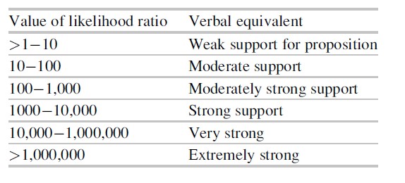
In the case of the DNA evidence with a likelihood ratio of 1,000, the expert would either report the numerical value of the likelihood ratio as such or would report that the DNA evidence provides “moderately strong” to “strong” support to hypothesis 1 (the suspect is the donor). The decision to use the numerical or the verbal form would depend on the extent to which the expert considers the data underlying the calculation of the likelihood ratio to be robust. This sounds like a sensible criterion. However, there are those who advocate the blanket use of verbal terms, i.e., even if perfectly valid qualitative empirical data are available, arguing that the use of a uniform reporting format is vastly preferable and adding that quantitative data are generally too complex for nonscientists to grasp.
The Prosecutor’s Fallacy
Regardless of the use of words or numbers, statements of the probability of the evidence under a particular hypothesis, as made in the Bayesian approach, are often prone to misunderstanding and may strike the recipient as counterintuitive. The finding that the similarities observed between the handwriting of the writer of an anonymous letter and the reference material produced by the suspect are much more likely if the suspect wrote the questioned sample than if it was written by a random member of the population is often taken to mean the converse: that it is much more likely that the suspect wrote the questioned handwriting sample than that it was written by a random member of the population.
However, if we do this, we are guilty of making a fundamental logical error which, in the judicial context, has come to be referred to as the prosecutor’s fallacy (Thompson and Schumann 1987). Although the term would seem to suggest that prosecutors are particularly prone to this fallacy, it is in fact an example of a more general type of error that is often made in the context of probability statements or inverse reasoning, where it is known as the “fallacy of the transposed conditional.” In its simplest form, it is easily spotted: if an animal is a cow, it is very likely to have four legs. However, the converse clearly does not hold: if an animal has four legs, it is not very likely to be a cow.
Transposed conditionals or prosecutor’s fallacies are very frequently encountered in the context of DNA evidence. Suppose a partial profile is obtained from a crime scene sample whose frequency in the relevant population is estimated to be smaller than 1 in 100,000. If the expert subsequently reports the probability that a random member of the population has the same profile as the crime scene sample as being smaller than, say, 1 in a 100,000, this statement is frequently understood to mean that the probability that the DNA does not originate from the suspect is smaller than 1 in a 100,000. However, the former is clearly a statement of the probability of the evidence (i.e., a match with the partial profile), while the latter is a statement of the posterior probability of the source hypothesis. Mathematically, the latter statement would be correct in a situation where the prior probability was set at 50 %, or 1 to 1. This would be the case if, in addition to the matching suspect, only one person would equally qualify as a possible donor, which will not frequently be a reasonable assumption to make. If, for the sake of the argument, the prior probability were set at 200,000 (e.g., the size of the adult male population of a large town), application of the odds form of the Bayes’ rule would yield a posterior probability of 33.3 %: (1 to 200,000) × 100,000 = 1 to 2, or 33.3 %.
Transposed conditionals may also occur in the context of cause and effect arguments. While it is correct to say that the street will be wet if it has been raining, the converse is clearly not necessarily true. The single observation that the street is wet does not allow us to infer that it must have been raining, or even that it has probably been raining. Alternative explanations are possible: The street may have got wet when the police used water cannon to break up a demonstration, or it is wet because somebody has just been washing his car. So we can make a statement about the likelihood of a particular finding (e.g., a wet street) under a particular hypothesis (“it has been raining”) but not about the probability of this same hypothesis merely on the basis of the finding that the street is wet. To determine the posterior probability that it has been raining, we need to combine the evidence of the wet street with the prior probability of rain. In England, the prior would be high, but in a country like Dubai, it would presumably be very low. The same evidence combined with vastly different priors may lead to very different posterior probabilities.
Controversy
The Bayesian approach is not uncontroversial. Its opponents frequently view its advocates as “believers” (Risinger 2012). More specifically, critics of the Bayesian approach object to the subjective nature of the prior probability, as well as to the use of likelihood ratios which lack an empirical basis. While the former criticism is clearly valid, it might be argued that the explicit consideration of the prior probability and the formulation of alternative hypotheses is a virtue in that it helps identify the relevant questions and prevents tunnel vision. The conclusion format propagated by the predominantly British Association of Forensic Science Providers is not unproblematic either, in that a phrase, like “the examination provides strong support for the proposition that X originates from Y,” will almost invariably be interpreted to mean that it is very likely that X originates from Y. Without due warning, logically correct conclusions of this type will almost inevitably tend to be mistaken for the logically flawed ones they are meant to replace.
A further problem is highlighted by a decision of the English Court of Appeal in R v T (2010). In it, the judges express sharp criticism of the report of a footwear expert, who, quite in line with the policy of the (now defunct) UK Forensic Science Service, had phrased his conclusion in verbal terms without making it clear to the judge or the jury that the verbal conclusion was based on a quantitative estimate of the frequency of the characteristics size, pattern, and wear as exhibited by the shoe mark found at the crime scene. The expert’s conclusion was formulated as: “(.. .) there is at this stage a moderate degree of scientific evidence to support the view that [the Nike trainers recovered from the appellant] had made the footwear marks.” However, as later appeared from case notes that were not added to the original report, the expert had calculated a likelihood ratio of 100, which number he had subsequently converted into the verbal phrase “moderate support,” in accordance with the scale presented above. In addition, counsel for the appellant pointed out to the Court of Appeal that in his testimony in court in response to questions by the defense, the expert had mentioned estimates of the relevant characteristics of the shoe mark which, when combined, would lead to a likelihood ratio of no less than 26,400, in which case the footwear evidence would have been much more incriminating (in verbal terms expressed as “very strong support”). The Court of Appeal’s judgment is perfectly clear:
The process by which the evidence was adduced lacked transparency. (…) it is simply wrong in principle for an expert to fail to set out the way in which he has reached his conclusion in his report.
The Court of Appeal continues:
(…) the practice of using a Bayesian approach and likelihood ratios to formulate opinions placed before a jury without that process being disclosed and debated in court is contrary to principles of open justice.
The ruling in R v T has led to various reactions, many (Berger et al. 2011; Evett 2011; Redmayne et al. 2011) but not all (Risinger 2012) in defense of the Bayesian approach. While one may disagree with some of the views expressed in the Court of Appeal judgment, recent research conducted in the Netherlands suggests that there is at least one other problem with the use of these “logically correct” conclusion formats. It appears that evaluative opinions expressed in the Bayesian format are likely to be misunderstood not only by defense lawyers and judges but also by forensic experts themselves. Participants in the study were asked to indicate for a variety of statements whether they were correct paraphrases of the Bayesian style conclusions that were used in a fictitious report. The study shows that a proper understanding of statements involving likelihood ratios by jurists is alarmingly poor. In order to be able to compare actual versus supposed understanding, participants were also asked to indicate how well they understood the Bayesian style conclusions of the reports on a scale from 1 (“I do not understand it at all.”) to 7 (“I understand it perfectly.”). The most worrying finding to emerge from the study is no doubt that not only did judges, defense lawyers, and forensic experts alike tend to interpret the conclusions of the submitted reports incorrectly but they combined their lack of understanding with a high degree of overestimation: They believed they understood the conclusions much better than in fact they did. This suggests that the continued use of Bayesian style conclusion formats or likelihood ratios requires a major educational effort if structural miscommunication between experts and triers of fact is to be avoided. Aitken et al. (2010) and Puch-Solis (2012) may be seen as attempts to meet this demand.
Conclusion
The findings of a comparative examination undertaken with a view to establishing the source of a particular trace or set of traces do not strictly allow the type of probabilistic source attributions, be they of a quantitative or verbal nature, that until recently were used by the vast majority of forensic practitioners. With the advent of forensic DNA analysis over the last decades and the widespread use of the conceptual framework associated with the interpretation of DNA evidence, awareness among forensic practitioners of other identification disciplines of the inadequacies of the traditional evidence evaluation paradigm has grown rapidly. Increasingly, this is leading to attempts to apply a logically correct way to express the value of the findings of a source attribution examination of trace material other than DNA by expressing the weight of the trace evidence in a way similar to that used in forensic DNA analysis. This takes the form of a so-called likelihood ratio. The concept is similar to that of the diagnostic value, a measure which has found wide acceptance in fields like medicine and psychology as a way to express the value of any diagnostic test result.
The concept of the likelihood ratio requires the consideration of the probability of the evidence under two competing hypotheses, one based on a proposition formulated by the police or the prosecution, the other based on an alternative proposition which may be based on a scenario put forward by the defense. As such, the Bayesian approach may be seen as a remedy against suspect-driven investigations, in which the police tend to focus on collecting evidence that will confirm the suspect’s involvement in the crime and ignores alternative explanations. By contrast, in a crime-driven investigation, the investigators base the direction of the investigation on the clues provided by the crime rather than by the person of the suspect and develop one or more scenarios based on the evidence rather than make the evidence fit a particular scenario.
Technical or scientific evidence derived from material traces such as DNA, finger marks, handwriting, fibers, footwear marks, or digital data derived from a hard-disk or a mobile telephone may be incompatible with a particular hypothesis that is central to a larger scenario and then effectively eliminate that scenario. More frequently, scientific evidence may be more or less likely to be found in one scenario than another and in this way may help discriminate between various scenarios. It is the consideration of the totality of evidence, both direct, witness and scientific evidence if available, which forms the basis for the ultimate decision made by the trier of fact.
Bibliography:
- Aitken C, Roberts P, Jackson G (2010) Communicating and interpreting statistical evidence in the administration of criminal justice: fundamentals of probability and statistical evidence. In criminal proceedings – Guidance for judges, lawyers, forensic scientists and expert witnesses, Royal Statistical Society, London
- Association of Forensic Science Providers (2009) Standards for the formulation of evaluative forensic science expert opinion. Sci Justice 49:161–164
- Berger CEH, Buckleton J, Champod C, Evett IW, Jackson G (2011) Evidence evaluation: a response to the court of appeal judgment in R v T. Sci Justice 51:43–49
- Broeders APA (2006) Of earprints, fingerprints, scent dogs, cot deaths and cognitive contamination: a brief look at the present state of play in the forensic arena. Forensic Sci Int 159(2–3):148–157
- Cook R, Evett IW, Jackson G, Jones PJ, Lambert JA (1998a) A model of case assessment and interpretation. Sci Justice 38(3):151–156
- Cook R, Evett IW, Jackson G, Jones PJ, Lambert JA (1998b) A hierarchy of propositions: deciding which level to address in casework. Sci Justice 38(4):231–239
- de Keijser J, Elffers H (2010) Understanding of forensic expert reports by judges, defense lawyers and forensic professionals. Psychol Crime Law 18(2):191–207
- Evett IW (2011) Expressing evaluative opinions: a position statement. Sci Justice 51:1–2
- Inman K, Rudin R (2000) Principles and practice of criminalistics: the profession of forensic science. CRC, Boca Raton
- Inman K, Rudin R (2002) The origin of evidence. Forensic Sci Int 126:11–16
- Kirk PL (1963) The ontogeny of criminalistics. J Crim Law Criminol Police Sci 54:235–238
- Kirk PL, Grunbaum BW (1968) Individuality of blood and its forensic significance. Leg Med Annu 289–325
- Popper KR (1959) The logic of scientific discovery. Hutchinson, London
- Puch-Solis R, Roberts P, Pope S, Aitken C (2012) Communicating and interpreting statistical evidence in the administration of criminal justice: 2. Assessing the probative value of DNA evidence. Royal Statistical Society, London
- Quetelet A (1870) Anthropome´trie ou Mesure des Differentes Facultes de l’Homme. Muquardt, Bruxelles R v T (2010) EWCA Crim 2439
- Raymond JJ, Walsh SJ, Van Oorschot RA, Roux C (2004) Trace DNA: an under-utilized resource or Pandora’s box? – A review of the use of trace DNA analysis in the investigation of volume crime. J Forensic Identif 54(6):668–686
- Redmayne M, Roberts P, Aitken CGG, Jackson G (2011) Forensic science evidence in question. Crim Law Rev 5:347–356
- Risinger DM (2012) Reservations about likelihood ratios (and some other aspects of forensic ‘Bayesianism’). Law Probab Risk 0:1–11
- Saks MJ, Koehler JJ (2005) The coming paradigm shift in forensic identification science. Science 309:892–895
- Saks MJ, Koehler JJ (2008) The individualization fallacy in forensic science evidence. Vanderbilt Law Rev 61:199–219
- Stoney DA (1991) What made us ever think we could individualize using statistics? J Forensic Sci Soc 31(2):197–199
- Thompson WC, Schumann EL (1987) Interpretation of statistical evidence in criminal trials: the prosecutor’s fallacy and the defence attorney’s fallacy. Law Hum Behav 11:167–187
- Thornton JI, Peterson JL (2002) ‘The general assumptions and rationale of forensic identification’ } 24–2.0–2.1. In: Faigman DL, Kaye DH, Saks MJ, Sanders J (eds) Modern scientific evidence: the law and science of expert testimony. West Publishing Co, St. Paul
- Thorwald JT (1965) The century of the detective. Harcourt, Brace & World, New York, first published in German as Das Jahrhundert der Detektive, Droemersche Verlagsanstalt: Zurich 1964
See also:
Free research papers are not written to satisfy your specific instructions. You can use our professional writing services to buy a custom research paper on any topic and get your high quality paper at affordable price.
ORDER HIGH QUALITY CUSTOM PAPER

Always on-time

Plagiarism-Free

100% Confidentiality
