Vector Autoregression Research Paper - Examples

This sample Vector Autoregression Research Paper is published for educational and informational purposes only. If you need help writing your assignment, please use our research paper writing service and buy a paper on any topic at affordable price. Also check our tips on how to write a research paper, see the lists of research paper topics, and browse research paper examples.

Vector auto regression (VAR) models were introduced by the macro econometrician Christopher Sims (1980) to model the joint dynamics and causal relations among a set of macroeconomic variables. VAR models are useful for forecasting. Consider a univariate autoregressive model—for example, an AR(1) Yt = ? + ?Yt – 1 + ?t —which describes the dynamics of just one random variable Y (i.e., national income) as a linear function of its own past. Based on this model, the forecast of national income will depend just on its past history. However, economic variables such as national income, employment, prices, money supply, interest rates, and so on interact with each other. For instance, movements in interest rates affect the level of employment, which in turn affects the level of national income. In this multivariate setting, the forecast of national income will be a function of a larger information set that combines not only the history of national income but also the histories of many other variables, such as interest rates and employment. A VAR is the generalization of the univariate autoregressive model to a vector of economic variables.

Definition

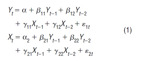
An n-variable vector auto regression of order p, VAR(p), is a system of n linear equations, with each equation describing the dynamics of one variable as a linear function of the previous p lags of every variable in the system, including its own p lags. A simple case is a VAR(2) (p = 2) for a vector of two variables (n = 2), say {Yt ,X

vectors auroregression form1

The innovations are assumed to be zero-mean random variables, E(?1t ) = E(?2t ) = 0, with constant variance, var(?1t ) = ?2 1 var(?2t ) = ?2 2, possibly correlated, cov(?1t , ?2t ) = ?12 ? 0, and with normal probability density functions.

The components of the definition are:

The n-dimension of the vector: number of variables to model, which is equal to the number of equations in the system.
The p-lag structure: identical number of lags for each of the n variables in the right-hand side of each equation.
The linear autoregressive specification.
The assumptions on the statistical properties of the innovations.

The joint dynamics are captured in two ways: (1) each variable is explained by the past history of every variable—Yt is a function of its own past and the past of the other variables in the system {Yt – 1, Yt – 2, … Yt – p , Xt – 2 , … Xt – p , …}; and (2) the innovations may be contemporaneously correlated, that is, ?12 ? 0.

Advantages

Easy implementation. Since every equation in the VAR has the same number of variables on the right-hand side, the coefficients {?1, ?2, …, ?11, ?21, …, ?11, ?21, … } of the overall system are easily estimated by applying ordinary least squares (OLS) to each equation individually. The OLS estimator has the standard asymptotic properties. In large samples, the OLS estimator is consistent and asymptotically normal distributed.

Classical inference. Since the OLS estimator has standard asymptotic properties, it is possible to test any linear restriction, either in one equation or across equations, with the standard t and F statistics. Suppose that one is interested in whether the second lag is relevant in the first equation. One writes the null hypothesis as H0: ?12 = ?12 = 0. This is a restriction involving only the first equation. It is also possible to test for restrictions involving more than one equation. Suppose that one is interested in whether the coefficients corresponding to Yt – 2 are identical across equations, that is, H0: ?12 = ?22. In both cases, an F-statistic will be appropriate.

The lag length p is also chosen by statistical testing or by minimizing some information criteria. Suppose that one starts by assuming p = 2. One writes the null hypothesis as H0: p = 2 against an alternative hypothesis p > 2, say Hy p = 3. The VAR model is estimated under the null and under the alternative, and testing is carried out by constructing either the F-statistic (based on the comparison of the sum of squared residuals for the restricted and unrestricted specifications) or an asymptotic likelihood test (based on the comparison of the value of the likelihood function for the restricted and unrestricted specifications).

Testing for Granger causality. It is of interest to know whether one or more variables have predictive content to forecast the variable(s) of interest. For instance, in system (1) one could ask whether X is helpful in predicting Y. The corresponding null hypothesis is that all the coefficients on the lags of X are zero, that is, H0: Yn = y12 = 0. If these coefficients are statistically zero, one says that X does not Granger-cause Y or, equivalently, X does not have any predictive content to forecast Y. The null hypothesis can be tested with a standard F-statistic.

Impulse-response function and variance decomposition. An important use of VAR is to quantify the effects over time of economic policy. Suppose that the monetary authority shocks interest rates. The questions become: When, for how long, and how much does the shock to interest rates impact employment and output? Impulse-response functions are designed to answer these questions. An impulse-response function describes the response over time of each variable in the VAR to a one-time shock in any given variable while keeping all others constant. For the system described in (1), one has four impulse-response functions: the impact and future effects on Y and on X of a unit shock to ?1, and the impact and future effects on Y and on Xof a unit shock to s2 .

Closely associated with the impulse-response function is the variance decomposition. This decomposition refers to the contribution of each innovation to the variance of the forecast error associated with the forecast of each variable in the VAR. Standard time series software provides both impulse-response functions and variance decomposition.

Shortcomings

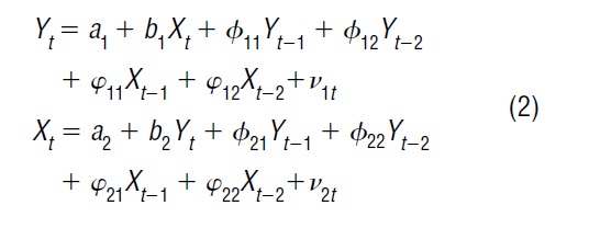
Ad hoc specification. VAR models are criticized because they do not shed any light on the underlying structure of the economy. Though this criticism is not important when the purpose of VAR is forecasting, it is relevant when the objective is to find causal relations among the macroeconomic variables. A structural VAR is a system of simultaneous equations that aim to analyze causal relations. For each variable in the system, there is an equation that accounts for simultaneous as well as dynamic interactions among the full set of variables. A structural VAR(2) for [Yf, X } corresponding to the system described in (1) looks like:

vectors auroregression form2

where v1 and v2 are known as the structural innovations. With matrix algebra, it is possible to solve for [Yf, Xf} in the structural VAR. The solution is known as the reduced form, which is the VAR in (1) subject to some parameter restrictions. The question becomes: Is it possible to recover the structural parameters from the estimated parameters of the reduced form? This is known as the identification problem. The structural VAR in (2) has fourteen parameters (twelve coefficients and the variances of the two innovations, assuming that the covariance is zero), while the VAR in (1) has thirteen parameters (ten coefficients, two variances, and one covariance of the innovations). To uniquely identify the structural parameters, the investigator needs one restriction on the structural VAR. Which restriction should be used?

Identifying restrictions. This is a point of debate in structural VAR modeling. The ideal view is that economic theory should dictate which restrictions to impose. However, Sims argued that economic theory was not informative about the appropriate identifying restrictions, and therefore the estimation of the reduced form was the most that one could accomplish. Some researchers impose restrictions on the coefficients of the contemporaneous variables (Sims 1980). Others impose restrictions on the covariance of the structural innovations (Hausman, Newey, and Taylor 1987), or on the long-run multipliers (Blanchard and Quah 1989).

The most popular identifying restriction is the recursive parameterization or lower triangularization of the matrix of contemporaneous coefficients. In the structural VAR(2) described in (2), this restriction is b1 = 0, which implies that exogenous shocks to Xwill not contemporaneously affect Y. If X is money and Y is output, the restriction b1 = 0 means that a shock to the money supply will not affect output instantaneously, though it will affect output with some delay depending upon the dynamics specified in the VAR model. The lower triangularization is the most popular restriction in the time series computer packages.

Ordering of the variables. When the innovations [s1t , e2t } are contemporaneously correlated, the impulse-response functions will depend on the ordering of the variables. A common solution is to transform the innovations (for instance, using the Cholesky decomposition) such that the transformed innovations are uncorrelated. The implication is that now one can trace the response of the system to an innovation shock in isolation without disturbing the rest of the innovations. The transformation also has implications for the specification of the system because now the first equation will have only one current innovation, the second equation will have two current innovations, the third equation will have three, and so on. Therefore, the ordering of the variables matters. There are no rules on how to choose the ordering of the variables. Economic theory may shed some light, but eventually the choice of the ordering will depend on the questions that the forecaster aims to answer.

Bibliography:

Blanchard, Olivier, and Danny Quah. 1989. The Dynamic Effects of Aggregate Demand and Aggregate Supply Disturbances. American Economic Review 79: 655–673.
Granger, Clive W. J. 1969. Investigating Causal Relations by Econometric Models and Cross-Spectral Methods. Econometrica 37 (3): 424–438.
Hamilton, James D. 1994. Time Series Analysis. Princeton, NJ: Academic Press.
Hausman, Jerry A., Whitney K. Newey, and William E. Taylor. 1987. Efficient Estimation and Identification of Simultaneous Equation Models with Covariance Restrictions. Econometrica 55 (4): 849–874.
Sims, Christopher. 1980. Macroeconomics and Reality. Econometrica 48 (1): 1–48.