Near Repeats and Crime Forecasting Research Paper

This sample Near Repeats and Crime Forecasting Research Paper is published for educational and informational purposes only. If you need help writing your assignment, please use our research paper writing service and buy a paper on any topic at affordable price. Also check our tips on how to write a research paper, see the lists of criminal justice research paper topics, and browse research paper examples.

It has been recognized for some time that crime clusters at a range of spatial scales. It is also well established that offenses cluster in time such that crime occurrence is more likely at particular times of the day, week, month, or year. More recently, a growing body of evidence has started to accumulate that indicates that crime also clusters in time and space, such that when an event occurs at one location, there is a temporary elevation in the probability that other events will occur nearby. Where crimes occur at the exact same location, this is referred to as repeat victimization, and where they occur at nearby locations, near-repeat victimization. Finding that the risk of crime diffuses in space has implications for crime forecasting. However, this type of work is in its infancy and naturally, many questions remain unanswered. For example, there is something of a disconnect in methodological terms between those techniques that are used to detect crime patterns and those that are, or should be, used to generate predictive crime maps. Moreover, approaches to calibrating predictive maps so that a range of factors can be incorporated, and so that the extent to which crime risk might be diffused varies across areas, are things that have received little or no attention. Similarly, the extent to which patterns of one type of crime might affect those of another largely remains unexplored in the literature. A final point is that while crime is known to cluster in space, analyses of crime at the street segment level suggest that there exist sharp discontinuities in risk from one street to another. As most methods of crime forecasting use some form of smoothing algorithm, this issue is not accounted for in these models. The above issues and how thinking about methods of crime forecasting might be developed to accommodate them are discussed in this research paper.

Introduction

Many things in life are random. Patterns of crime are not. Crime clusters at places, where places represent neighborhoods, street segments, or individual properties (for a review, see Johnson 2010). For many crimes, it is also evident that the timing of victimization is not random, with there being seasonal variation in the frequency of occurrence of offenses (Farrell and Pease 1994), and variation throughout the day (Ratcliffe 2002). Moreover, for burglary events, the elapsed time between events at the same home is typically short (Johnson et al. 1997). More recently, using (for example) techniques originally developed to detect disease contagion, research has examined the association between the timing and location of crimes committed not just against the same target but also those nearby. The finding so far consistently observed is that when a crime occurs at one location, others are more likely to take place swiftly nearby. This finding applies to volume crime such as burglary, but also extends to other event types such as shootings (Ratcliffe and Rengert 2008) and insurgent activity (Townsley et al. 2008). In this research paper, research concerned with this phenomenon – referred to as near-repeat victimization – is reviewed and consideration is given as to how this area of investigation informs methods of crime forecasting, and how it might usefully evolve. The paper is organized as follows. It begins with a discussion of methods of quantifying repeat and near-repeat victimization. Next, theoretical explanations as to why such patterns might emerge are considered. In the subsequent section, a number of unanswered research questions that might inform future work are identified. And, finally, there is a discussion of how what is already known has informed methods of crime forecasting and how such methods might be developed.

Fundamentals: Identifying And Quantifying Patterns Of Near Repeats

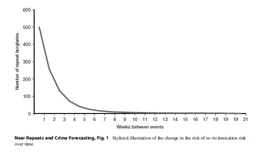
A number of techniques have been used to examine patterns of repeat victimization of the same home (in the case of burglary) and near-repeat victimization. In the case of the former, the approach to analysis is somewhat simple. For repeat victimization proper, an incident of repeat victimization is defined simply as an offense where the victim has previously experienced an incident of the same type (or, crime more generally depending upon the researcher’s interest). For this type of analysis, one may calculate the time elapsed between events and summarize this interevent distribution. A typical finding is that the time elapsed between offenses is short, with the count of events declining logarithmically as a function of time. Figure 1 gives an example of such a time course (in this case, using fictional data).

Near Repeats and Crime Forecasting Research Paper

One may also estimate whether the number of homes that were observed to have been victimized one, two, three, or more times differs from chance expectation, assuming that events are independent. The approach to analysis typically used is to estimate the number of homes that would be expected to be victimized 1 to N times, assuming the observed distribution can be explained by a Poisson process (the null hypothesis in this case). This type of analysis can be conducted assuming that the overall risk to homes is homogeneous or that there will be variation at the area (Trickett et al. 1992), neighborhood or house-level (Johnson 2008). A similar approach can also be used to estimate the expected time course of repeat victimization (Johnson 2008). In the case of burglary, what the available evidence – conducted across a variety of countries – suggests is that, relative to the pattern expected, the risk of victimization is temporarily elevated following an offense.

In terms of near-repeat victimization, the approach to analysis is slightly more complicated in that the analysis is extended to an examination of any regularity in the patterning of crimes that occur not just at the same locations, but also nearby. A number of approaches to analysis have been adopted. In one study (Bowers and Johnson 2005), using data recorded by the police (Merseyside, UK) that covered an interval of 5 years, the authors identified every street on which two or more burglaries had occurred. For each burglary, they then calculated how many doors apart that burglary had occurred from the most recent burglary that had also taken place on the same street. A distribution was then derived to indicate how many sequential burglaries had occurred one-door apart, two-doors apart, and so on. This distribution was standardized to account for the fact that because roads are not infinite in length, there would be more opportunities for burglaries to occur (say) one-door apart from each other than (say) 30 doors apart. The results clearly indicated a pattern of distance decay, such that when burglaries occurred on the same street as each other, they were most likely to occur near to each other. Further analyses also indicated that burglaries that occurred on the same street were also more likely to occur on the same side of the street as each other and near to each other in time. Thus, when a neighbor of a victimized home was burgled, this was more likely to occur within 1 week of the first offense than (say) 7–14 days apart.

Such analysis examines patterns observed on the same street, but does not consider those offenses that occur near to each other but on a different road. For this reason, other methods of analysis, originally developed to detect disease contagion, have also been used. A number of studies have used a technique developed by Mantel (1967). This test is used to see whether crimes that occur closest to each other in space are also more likely to occur close to each other in time. This particular test provides a single index of space-time clustering for a particular area, and while it has useful diagnostic value, it is a relative measure which means that what is defined as near (in time or space) is not actually specified. That is, space-time clustering would be detected even if it were the case that the events that were closest to each other were (say) two miles apart, if that is, relative to events that occurred further apart, these crimes also tended to occur closest to each other in time.

A test developed by (Knox 1964) provides an alternative approach. In this case, each event of interest is compared with every other and the absolute distance and time elapsed between them is computed. In the original formulation, a 2×2 contingency table was populated to enumerate how many pairs of events had occurred close to each other in space and time; close in space but not in time; close in time but not space; and neither close in space nor time. This test allows the researcher to define what is meant by “close” in both dimensions and hence provides more precise insight into observed patterns. To determine whether the latter differ from chance expectation, assuming the timing and location of events are independent, the expected counts are calculated for each cell by multiplying the total counts for the relevant row and column and then dividing by the total across all cells of the table (the same approach used to compute expected counts for a Chi-Square statistic).

Such an analytic strategy may be sufficient for estimating the extent to which a disease is contagious, and for examining general patterns in the space-time dynamics of crime, but it does not provide a particularly precise picture of crime patterns. This is so because only two categories of near and far are defined. For this reason, in recent work (Johnson and Bowers 2004a), the approach has been extended so as to include numerous categories. In general, around 10–20 different spatial and temporal bandwidths have been used. For example, Johnson and Bowers (2004a) used spatial bandwidths of 100 m and temporal intervals of 7-day periods. Patterns observed across these relatively finely resolved categories can then be compared with each other and with a more general “distant” category.

One potential weakness with the approach to statistical inference used for this test is that the test statistics are based on parametric assumptions that might not be met. For this reason, Johnson et al. (2007a) developed a nonparametric version of the test that uses a Monte Carlo simulation to estimate the statistical significance of observed patterns. As was the case for previous work, the authors found that burglary clustered in time and space more than would be expected if the timing and location of events were independent. Importantly, in that study, the authors found consistent patterns within each of two cities in each of five different countries, suggesting that the patterns are not specific to a particular locality.

A further refinement in the existing research involves a more precise study of the distribution of space-time clusters. To elaborate, for the techniques discussed above, the approach to analysis involves counting the number of pairs of events that occur within particular spatial and temporal intervals of each other and comparing these counts to expectation, assuming that the timing and location of events are independent. In an early study, Johnson and Bowers (2004b) extended the approach by examining whether pairs of events that occur close to each other in both space and time also cluster. They did this by computing the number of event pairs (hereafter, close pairs) that occurred within a given space and time interval (100 m and 1-month) of each other for a series of 151 neighborhoods, for each month of a 1-year period. Their analyses showed that in general, the number of close pairs that occurred in a neighborhood was similar for sequential monthly intervals, but that the correlation was lower and typically nonsignificant where the counts for intervals that were more than one month apart were compared. Similarly, it was evident that if a neighborhood had a high count of close pairs in a particular month, those nearby also tended to also have a high count of close pairs around the same time. There was no systematic association between the count of close pairs in neighborhoods that were a fair distance apart, regardless of whether comparisons were made for the same month or other intervals.

A slightly different approach was adopted in other work (Johnson et al. 2007b). In that study, for each burglary event, the authors calculated how many other burglaries had previously occurred nearby in the recent past. The idea of doing so was to estimate the number of events that might typically make up a spate (or polyorder chain) of burglary events. In a further study, this time concerned with Improvised Explosive Device (IED) attacks in Iraq, Johnson and Braithwaite (2009) used a Monte Carlo method to compare the observed length of spates with those expected, assuming that the timing and location of events were unrelated. In this study, relative to expectation, it was apparent that while there were significantly more spates that comprised six or more IED attacks, there were actually significantly fewer spates with seven or more offenses. That is, after six IED attacks had occurred at or near to a location shortly after each other, others were actually less likely to occur than would be expected if the timing and location of attacks were independent. Collectively, these findings suggest that when a crime occurs at a location, others are more likely to occur nearby in the near future. However, as time elapses, this increase in risk decays.

Following the development of methods to quantify patterns of near repeats, a number of studies have been conducted. Between the period 2003 and 2011, more than 30 studies of which the authors are aware have so far been published on this topic and so what should be apparent is that while the analysis of this type of patterning for crime events is relatively new, there now exists a considerable body of research for a range of different types of event and for different countries.

Possible Explanations For Near-Repeat Patterns

Much of the research concerned with spatial patterns of crime ignores the dimension of time, focusing exclusively on spatial patterns aggregated over some interval. Such analysis might be described as examining the stable or slow dynamics of crime. In contrast, research concerned with near repeats explicitly examines both spatial and temporal patterns, and does so at a fairly fine level of resolution. As such, this kind of analysis might be described as examining the fast dynamics of crime.

One question that remains unanswered is how the fast and slow dynamics of crime influence each other. For instance, do the fast dynamics give rise to the slow ones, or vice versa, or, is the association more complex? Given that many hotspots endure it would seem unlikely that the fast dynamics entirely define the slow ones, and so disentangling this issue is of clear importance. Controversies such as this will be discussed in a later section.

Apropos why repeat and near-repeat victimization occur, two theories have been proposed to explain observed patterns. According to the first, variation in enduring characteristics that makes targets vulnerable to crime explains the patterns described. This concept of risk heterogeneity (see Johnson 2008) assumes that – other than the target involved – there is no association between one offense and another. The risk of victimization across targets is seen as being time-stable and a function of a set of characteristics that many or all offenders would find appealing.

Considering offender spatial decision making, research has generally focused on the types of place that offenders might display preferences for. Underlying such models is the idea that offenders, like the rest of the population, are rational decision makers (Clarke and Cornish 1985) who weigh up the benefits, costs, and effort associated with possible courses of action. Such decision making is not seen as involving a comprehensive evaluation but is regarded as being more heuristic in nature, with offenders using “rules of thumb” to assess opportunities perceived. Of course, offenders will rarely be aware of the true costs, benefits, and rewards of any particular decision made, and so their decision making is instead considered to be bounded by the information of which they are aware, cognitive biases, and so on. However, the point of central importance is that in most of the research literature, offender decision making is typically considered in terms of spatial choices. These may be hierarchical, insofar as certain types of areas may first be selected, after which particular targets – which may confirm to cognitive templates – are selected, but they are nonetheless spatial.

Research on near repeats draws more explicit attention to the dynamic nature of offender spatial decision making. For example, the offender as forager hypothesis (Johnson and Bowers 2004b; Johnson et al. 2009b) borrows from concepts regarding animal foraging, ideas that are well established within the field of ecology. The obvious reason for the comparison being that the activities considered, be they animal foraging or offender decision making, share common underlying goals. Both seek to maximize benefits, while minimizing expended effort and the associated risks (be it detection or being eaten). Moreover, both forms of activity are subject to constraints. The actor, be it animal or offender, can only move so far and so fast per unit time, and both expend effort in doing so. In neither case would it seem to be efficient to make future choices without reference to previous ones, particularly those made most recently. Where recent choices have been rewarded, their repetition would seem reasonable, albeit up to a certain point. In the case of the offender, returning to the same location repeatedly would likely ultimately either lead to arrest or little reward – as little would be left to take. The targeting of locations near to successfully exploited targets may represent an efficient strategy as the first law of geography (Tobler 1970) states that things that are close to each other are more similar than are those that are far apart. Thus, nearby targets are likely to share important features (e.g., levels of natural surveillance, escape routes, etc.) of those previously successfully targeted that will make them good opportunities for crime, at least in the short term. The latter point is important as things may be subject to change, and memory fades.

Thus, in contrast to theories of risk heterogeneity, those concerned with event dependency (Pease 1998) assume that victimization influences future risk. In the case of crimes such as burglary, where the conditions at already targeted locations are conducive to crime, it is hypothesized that the same offender (or group of offenders) will return and that they will do so swiftly.

A number of research methods have been used to test the two types of theory. The analysis of crimes detected by the police (Bernasco 2008; Johnson et al. 2009b) indicates that, relative to burglaries that occur close in space or time to each other, those that occur nearest to each other in both dimensions are massively more likely to be the work of the same offender(s). The same is true for theft from motor vehicles (Johnson et al. 2009b). Such patterns would be predicted by the offender as forager hypothesis but are inconsistent with theories of risk heterogeneity.

Interviews with offenders also suggest that offenders return to the same locations (Ashton et al. 1998) and those nearby (Summers et al. 2010) for reasons compatible with the offender as forager hypothesis. Of course, such research also indicates that target attractiveness plays a role; an offender can only return to an area or street they have already targeted, and so as a minimum, risk heterogeneity will play a role in determining where offenders commit initial offenses. Moreover, not all offenders will adopt foraging strategies and for such offenders, target attractiveness may be the primary factor that they consider when selecting targets.

In the case of repeat burglary victimization, it is apparent that relative to low frequency offenders, prolific offenders who are more established in their criminal careers appear to be more likely to return to the exact same properties (Everson and Pease 2001). It is unclear whether the same applies to those who commit near repeats, but this would seem to be plausible. If this is the case, then it would suggest that target attractiveness (risk heterogeneity) alone may explain the targeting strategies of those burglars who infrequently commit crime, but that those who routinely engage in such offenses, the experiences associated with the burglaries they have recently committed will significantly inform their subsequent choices.

A different approach to theory testing and falsification than has been discussed hitherto uses mathematical models or computer simulation. The detail is not important, but the central idea is to see if models that describe a particular data-generating process – such as event dependency or risk heterogeneity – are sufficient to generate space-time patterns of events that resemble those observed in crime data. This research indicates that models that include only – or completely exclude – risk heterogeneity are incapable of generating the time course of repeat victimization (Johnson 2008) or nearrepeat victimization (e.g., Pitcher and Johnson 2011). However, those that include both processes generate patterns much like those observed in the research described above.

Mohler et al. (2011) have also used a class of statistical model, originally developed to examine patterns of earthquakes, to examine patterns observed for the crime of burglary. The aim of this type of statistical model, known as a self-exciting point process, is to estimate the contribution of (unobserved) time-stable factors that vary across space (e.g., the location and size of unknown fault lines in the case of earthquakes) and the effects of after-shocks that follow each quake. Using data for burglaries recorded by the police in Los Angeles, Mohler et al. (2011) find that for this event type at least, both types of process are important. Thus, it would seem that both types of explanation – risk heterogeneity and event dependency – have a part to play.

Before leaving this discussion, it is worth noting that one methodological issue that is sometimes discussed with respect to patterns of repeat or near-repeat victimization is that these might be explained by an artifact associated with the data. It is widely acknowledged that police-recorded crime data is by no means a perfect measure of crime, as much crime goes unreported. Moreover, from the perspective of when crimes occur, it is often difficult to pinpoint the exact time of a burglary as this will be unknown and so estimation procedures are often necessary. However, these issues are unlikely to influence the results of the types of analysis discussed unless there is a systematic pattern (in space and time) associated with them, and there is no reason to suspect that there is.

A potentially greater concern involves edge effects. In the case of near-repeat victimization, burglaries that occur at or near the boundary of a study area have more opportunity to be further away from other burglaries than do those in the middle; likewise, burglaries that occur at the start of a time period have more potential to be further apart in time from other crimes than do those that occur at the end. However, because the expected distribution of events is established using the observed data and methods such as the Monte Carlo procedure discussed above, we suggest that the approach to analysis accounts for edge effects (and other issues).

What Don’t We Know About Near-Repeat Patterns?

Although much has been learned about near repeats over the last 8 years, a number of things are currently unclear. For example, while the research to date suggests that both theories of risk heterogeneity and event dependency have a part to play in explaining space-time patterns of crime, the precise contributions of each process are not well understood. For instance, as discussed, in the case of burglary, it could be that some burglars tend to select targets purely on the basis of their perceived attractiveness, whereas others select targets in a way that is consistent with the optimal foraging theory discussed above. Others still may adopt a more even mix of strategies. An alternative explanation is that all offenders adopt the same strategy, but that some burglary events encourage a swift return to the same property or those nearby, whereas in other cases, the reverse is true. For instance, if an offender is challenged by a resident while attempting to burgle a home, that offender is likely to be discouraged from returning to the same neighborhood for some time. To put it another way, at what unit of analysis – the offender or the event – do these two types or processes (risk heterogeneity and event dependency) operate?

The preceding discussion focused on the crime of burglary, but as is evident in the introduction to this research paper, near repeats are observed for a range of event types and it is likely that different mechanisms will be responsible for observed patterns for some of these. In the case of similar crimes, common explanations may suffice but is the same true for very different types of events?

While this seems unlikely, there may be some commonalities associated with human mobility dynamics. For instance, most actors are subject to constraints that limit how far they can travel per unit of time and how fast they can do so. It may also be reasonable to assume that actors are more likely to engage in activities at locations with which they are familiar than those that they are not, regardless of the event type. However, while there may be some commonalities in the explanations for different event types, understanding the differences will be important if the patterns are to be truly understood.

Little research has considered how patterns, and the contribution of the two theoretical processes (risk heterogeneity and event dependency) discussed, might vary across space and/or time, but there are two exceptions. Townsley, Homel, and Chaseling (2003) found differences in patterns of repeat and near-repeat victimization across a sample of five different suburbs and found that near-repeat victimization was more likely in those suburbs with more homogeneous types of housing. They interpret this as suggesting that where replicas of a previously victimized home exist, offenders will be more likely to commit near repeats. Bowers and Johnson (2005) examined patterns of repeat and nearrepeat burglary victimization for a larger sample of 118 areas in one county in the UK. They found the former to be accentuated in deprived areas, but that patterns of the latter were clearer in affluent ones. However, other than these two early studies, little research has examined how patterns vary across spatial units, or if they are stable over time. It is possible, for example, that in one hotspot of criminal activity, there may be a strong pattern of near repeats, whereas in another, there will be no such pattern. Moreover, patterns of near repeats may ebb and flow over time, perhaps with the seasons (Johnson and Bowers 2004b) or perhaps as a consequence of certain types of offenders moving into or out of an area. Studying such dynamics is likely to inform understanding and assist in efforts of crime forecasting.

Given previously well-documented offender versatility, it may be expected that the space-time distribution of different types of offense would be correlated. Only one study (Johnson et al. 2009b) has so far examined near-repeat patterns across offense types. In that study, patterns of burglary and theft from vehicle were considered and it was found that for the two types of event, patterns of victimization were not correlated in space and time. Further analyses of crimes detected by the police for the same area indicated that offenders who committed one type of offense typically did not commit offenses of the other kind. This latter finding explains why the space-time distributions of the two types of offenses were not found to be correlated, but are at odds with other research concerned with offender versatility. Thus, it is not yet clear whether the finding regarding space-time clustering across offense types is typical across other localities or if it holds true for other combinations of offense types.

Another issue which requires attention is how co-offending or offender cooperation might contribute to (or interfere with) patterns of repeat or near-repeat patterns. Empirical research on co-offending more generally is in its infancy (Andresen and Felson 2010) and so this may be a particularly useful area to consider. For example, it is possible that offenders may share information regarding good opportunities, or (for example) work streets together in some cases. If this is the case, then the “boost” hypothesis would still explain observed patterns, but establishing the extent to which offenders cooperate in this way would inform criminological understanding and have implications for police practice. An alternative is that where offenders work together, the patterns are quite different to when they offend alone. Those that co-offend may adopt quite different strategies to the foraging approaches discussed above. Regardless of the reality, it would be beneficial to examine this.

A point that is discussed below concerns what the appropriate units of analysis for research of this kind should be. For the Knox and similar forms of analysis, the distance between events is measured using either the Euclidian (straight-line distance) or Manhattan (the sum of the difference between two points in the horizontal and vertical dimensions) distance between them. Given that many offenses occur along a street, this may be inappropriate or it may mask important variation. For example, two homes may be (say) 100 m from each other in Euclidian space, but be separated by a much more substantial distance along the street network. Thus, a further question that has not been addressed to date is how risk spreads along the street network as opposed to within streets or across Euclidian space. Researchers might ask if risk spreads preferentially from streets that are connected to each other, if such a diffusion of risk is more likely along similar types of streets, and if there are other regularities associated with when risk spreads from one street to another and when it does not.

Predicting Future Crime Locations

While there is still much that is unknown about space-time patterns of crime, current findings have practical application and inform criminological theory. The finding that following one crime at a particular location, the risk of others occurring nearby is temporarily elevated has obvious implications for crime prevention and crime forecasting. In this regard, recent work has examined the forecasting accuracy of simple mathematical models that take account of both the timing and location of historic events, and compared this with methods that consider only where historic events occurred (regardless of when they took place). For both types of model, the risk of crime is assumed to be a function of how much crime previously occurred at that location and nearby. In the case of models that take account of when and where crimes occurred, the reason is that the risk of crime is assumed to diffuse in space much like a contagious disease. And, consequently, more recent events are seen as more important and thus given a larger mathematical weighting in the models. In the case of those models that do not consider the timing of events, the theoretical rationale for considering the location of events that occurred near to, as well as at, each location has not been explicitly articulated, but the research concerned with near-repeat victimization at least provides a justification for this.

A typical method of contrasting the accuracy of such models may be described as follows. First, a study area is represented by a grid of regular sized cells (say 50 m by 50 m in dimension). Second, predictions are generated for each cell using data for a training interval. To calculate the expected risk in each cell, a mathematical formula is used which considers how much crime occurs in each cell and within some (usually) fixed distance from it. What that distance or bandwidth is often is selected for atheoretical reasons, such as the visual elegance of the resulting map. However, the research concerned with near repeats provides a theoretically meaningful way of determining the bandwidth. For example, the Knox analysis can be used to determine the distance and time over which the risk of crime appears to diffuse in space and time, and hence, the distance and time over which each crime might be expected to affect the risk of crime at nearby locations. Regardless of the approach to selecting the bandwidth, all of the methods typically apply a weighting to each event that is inversely related to the distance the event occurs from the center of the cell. Methods that take account of the timing of events additionally apply a weighting that considers when the events occurred. In this case too, a bandwidth is selected and the weighting applied to events within that bandwidth is usually inversely related to the time elapsed between that event and the period for which the forecast is generated.

After generating predictions for a particular model, these are compared with observed outcomes for a series of subsequent forecast intervals. In the analyses so far conducted (e.g., Bowers et al. 2004; Johnson et al. 2007b, 2009a) for the crime of burglary, those models that take account of both the timing and location of burglary outperform those that consider only the location of previous events. In a recent study, Mohler et al. (2011) show that statistical methods that explicitly estimate the likely contributions of time-stable (estimated using crime data alone) and event-dependent processes improve the forecast accuracy of such methods.

Other work (e.g., Johnson 2008) has examined how forecasting models can be improved by considering time-stable characteristics of the environment in a different way. In that study, the researchers incorporated simple data regarding the distribution of potential targets (houses) of burglary and the street network. Again, improvements in forecast accuracy were observed relative to models that exclude such information.

Future Developments In Prediction

Work on predictive analysis is, however, embryonic. For example, information on the street network has so far been limited to an indication of where roads are physically located. As discussed above, the risk of crime may diffuse along the street network in particular ways. Even in the most basic sense, if risk diffuses along the street network rather than through geographical space, then the topology (the ways in which segments of the street network are or are not connected to each other) of the network may significantly affect how the risk of crime spreads. For example, if two cells in an area were near to each other but not connected by the street network, then it is possible that risk may not diffuse between them, or that any propagation is impeded relative to two homes that are the same distance apart but connected (all other things being equal). In addition, even if two cells are connected via the street network, while they might be close in Euclidian space, they may be far apart in topological terms. The extent to which a consideration of topology might play a role in improving the accuracy of crime forecasting is currently unknown but amenable to mathematical analysis.

As discussed above, the way in which crime risk might spread in space and time might well vary across different neighborhoods. In the analyses so far conducted, patterns are modeled in the same way across areas and so gains in predictive accuracy might be achieved by systematically studying how patterns vary across areas and incorporating such findings into predictive models. Similarly, patterns might vary in time. For example, near repeats might be more likely at certain times of the day or even the year. Such variation is plausible as the risk of crime more generally is known to fluctuate throughout the day (Ratcliffe 2002) and year, presumably reflecting (amongst other things) variations in people’s routine activities and hence their availability to act as capable guardians against crime. In line with this suggestion, Johnson et al. (2007) find that when pairs of events occur near to each other in both space and time, they are more likely to occur during the same interval of the day than chance expectation. However, with the exception of this study, no research of which of the authors are aware has examined how the risk of near-repeat victimization might vary over the course of the day and how predictable patterns might be.

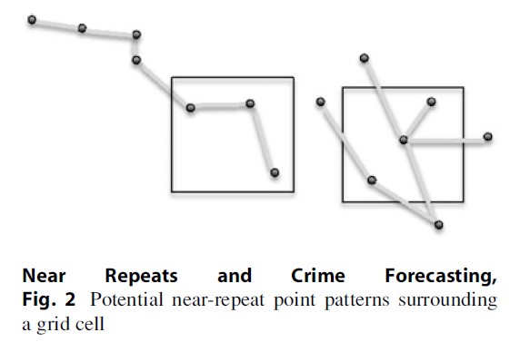
One issue not so far discussed is that the types of analyses generally conducted to detect patterns of space-time clustering focus on point patterns (the precise locations of crime events), whereas the methods used to generate predictions do so with reference to a fixed grid. The potentially important issue is that for point patterns, space time clustering may be generated in a number of ways. For example, space-time clustering might occur if many pairs of events happen close to each other in space and time and are all located in an area surrounding a single cell – let us refer to this as cell A. Space-time clustering might also occur if sequential pairs of events happen near to each other but if, over time, the pairs of events generally move away from cell A. Figure 2 represents these possibilities. It should be clear that the risk to cell A should be modeled differently if the first type of pattern were typical than if the second type were dominant. However, it is not possible to differentiate between these two types of directional pattern using the kinds of analyses that have been traditionally used.

Near Repeats and Crime Forecasting Research Paper

There appears to be value in matching units of analysis used to determine space-time patterns with those used in prediction. In two recent papers (Mohler et al. 2011; Rey et al. 2011) concerned with space-time clustering, the units of analysis were grid cells rather than point locations. For example, Rey et al. (2011) divided their study area into ¼ by ¼ mile grid cells and calculated how many burglaries occurred in every cell each month for a period of 51 months. Next, using a discrete Markov Chain framework, for each month, they examined the probability with which each cell would transition from a state of experiencing no burglaries or a state of experiencing at least one to the same or the alternate state. Consistent with research that has examined point patterns, their findings clearly showed that the state of a cell (whether crimes occurred in it or not) at any interval was positively associated with the state of that cell and those adjacent in the previous period. Moreover, that this pattern could not be explained by risk heterogeneity alone. This, or similar approaches, may help to more precisely calibrate methods of crime forecasting that take account of both the timing and location of events.

In addition to the issue of matching units of analysis for description and prediction, there is still the underlying question of what the relevant unit of analysis should be in crime forecasting of this kind. Grid-based predictions are largely used because of computational convenience. That is, constructing a grid of regular sized cells is straightforward and the spatial relationship between each cell and every other is simple to establish. However, crimes do not occur on a grid (except where the street network is of that geometric configuration), and offenders are unlikely to engage in decision making with reference to such a representation of the world. Moreover, research suggests that there are sharp discontinuities in the distribution of crime risk, such that (for example) two roads that are very near to each other (even directly connected) may experience very different risks (Groff et al. 2010). Possible reasons for this variation are numerous but the point of central importance is that – whatever the explanation – something about the way those street segments differ is associated with variation in crime risk. This is also true of block faces in a US context which in essence are equivalent to street segments in Europe. Where risk is modeled on a grid surface, this variation is ignored as the grid cells are unlikely to reflect the geometry of the street network. Thus, the risk for the cell represents the average risk across those street segments within it, even though the places within the cell may differ considerably in factors including crime risk. Moreover, the smoothing algorithms used to derive grid-based predictions will mean that risk is assumed to diffuse from one location to any another nearby location, irrespective of the characteristics of the type of location, something that may be unreasonable.

Thus, it is suggested that future research should explore methods of crime forecasting using street networks or block faces rather than grid cells. Methods of describing and representing street networks are possible using basic techniques from a branch of mathematics known as graph theory, and that exploring this type of approach is an obvious next step in the research agenda.

In closing, a further question to consider as yet unasked in the research literature is precisely what does one want to predict with forecasting models? To make things concrete, consider those forecasting models developed to predict patterns of burglary. As discussed, the available evidence suggests that observed patterns are most likely the result of two data-generating processes: risk heterogeneity and event dependency. If, as has been tentatively suggested, these two processes reflect the dominant targeting strategies of two different types of offender, the patterns and locations of offenses generated by one group of offenders might differ from those of the other. If so, should the accuracy of forecasting models be evaluated with respect to the total amount of offenses correctly predicted, or should such assessment also consider what types of events (e.g., near-repeat victimizations) are accurately identified? One reason for asking such a question is that the types of crime reduction action that might be triggered by the two types of prediction – those that might forecast the locations of events most likely committed by those who adopt foraging strategies as opposed to those who adopt more opportunistic strategies – may well differ. If this proves to be the case, for events that may be considered most likely the result of the consequence of enduring characteristics of places (assuming such a distinction is possible), situational crime prevention interventions will likely represent the most productive approaches to crime reduction. In contrast, where events predicted are more likely to be the work of offenders who adopt optimal foraging strategies, efforts directed toward detecting (or preventing) future offenses will likely prove more fruitful. In operational terms, the development of methods of forecasting that are specifically tailored to these two types of policing may be more helpful than are those models that predict more offenses (of any kind). The extent to which this is true is, of course, an empirical question.

Bibliography:

Andresen MA, Felson M (2010) The impact of co-offending. Br J Criminol 50(1):66
Ashton J, Brown I, Senior B, Pease K (1998) Repeat victimisation: offender accounts. Int J Risk Secur Crime Prev 3:269–280
Bernasco W (2008) Them Again? Same-Offender Involvement in Repeat and Near Repeat Burglaries. Eur J Criminol 5(4):411–431
Bowers KJ, Johnson SD (2005) Domestic burglary repeats and space-time clusters. Eur J Criminol 2(1):67
Bowers KJ, Johnson SD, Pease K (2004) Prospective hot- spotting. Br J Criminol 44(5):641
Clarke RV, Cornish DB (1985) Modeling offenders’ decisions: a framework for research and policy. Crime Just 6:147
Everson S, Pease K (2001) Crime against the same person and place: detection opportunity and offender targeting. Crime Prev Stud 12:199–220
Farrell G, Pease P (1994) Crime seasonality: domestic disputes and residential burglary in Merseyside 1988–90. Br J Criminol 34(4):487
Groff ER, Weisburd D, Yang SM (2010) Is it important to examine crime trends at a local “micro” level?: a longitudinal analysis of street to street variability in crime trajectories. J Quant Criminol 26(1):7–32
Harries KD, Stadler SJ, Zdorkowski RT (1984) Seasonality and assault: explorations in inter-neighborhood variation, Dallas 1980. Ann Assoc Am Geogr 74(4):590–604
Johnson SD (2008) Repeat burglary victimisation: a tale of two theories. J Exp Criminol 4(3):215–240
Johnson SD (2010) A brief history of the analysis of crime concentration. Eur J Appl Math 21(4–5):349–370
Johnson SD, Bowers KJ (2004a) The burglary as clue to the future. Eur J Criminol 1(2):237
Johnson SD, Bowers KJ (2004b) The stability of spacetime clusters of burglary. Br J Criminol 44(1):55
Johnson SD, Braithwaite A (2009) Spatio-temporal modelling of insurgency in Iraq. Criminal Justice Press, New York
Johnson SD, Bowers K, Hirschfield A (1997) New insights into the spatial and temporal distribution of repeat victimization. Br J Criminol 37(2):224
Johnson SD, Bernasco W, Bowers KJ, Elffers H, Ratcliffe J, Rengert G, Townsley M (2007a) Space–time patterns of risk: a cross national assessment of residential burglary victimization. J Quant Criminol 23(3):201–219
Johnson SD, Birks DJ, McLaughlin L, Bowers KJ, Pease K (2007) Prospective crime mapping in operational context, final report. Home Office online report, London, UK, 19, 07–08
Johnson SD, Bowers KJ, Birks DJ, Pease K (2009a) Predictive mapping of crime by ProMap: accuracy, units of analysis, and the environmental backcloth. In: Weisburd WBD, Bruinsma G (eds) Putting crime in its place. Springer, London, pp 171–198
Johnson SD, Summers L, Pease K (2009b) Offender as forager? A direct test of the boost account of victimization. J Quant Criminol 25(2):181–200
Knox G (1964) Epidemiology of childhood leukaemia in northumberland and durham. Brit J Prev Soc Med 18:17–24
Lockwood B (2012) The presence and nature of a near-repeat pattern of motor vehicle Theft. Secur J 25:38–56
Mantel N (1967) The detection of disease clustering and a generalized regression approach. Cancer Res 27(2 Pt 1):209
McGloin JM, Sullivan CJ, Piquero AR (2009) Aggregating to versatility? Br J Criminol 49(2):243–264
Mohler G, Short M, Brantingham P, Schoenberg F, Tita G (2011) self-exciting point process modeling of crime. J Am Stat Assoc 106(493):100–108
Mohler GO (2011) Self-exciting point process modeling of crime. J Am Stat Assoc 106:100–108. doi:10.1198/ jasa.2011.ap09546
Morgan F (2001) Repeat burglary in a Perth suburb: indicator of short-term or long-term risk? Crime Prev Stud 12:83–118
Pease K (1998) Repeat victimisation: taking stock. Home Office, London, p 48, ISBN 1-84082-089-6
Pitcher AB, Johnson SD (2011) Exploring theories of victimization using a mathematical model of burglary. J Res Crime Delinq 48(1):83
Ratcliffe JH (2002) Aoristic signatures and the spatiotemporal analysis of high volume crime patterns. J Quant Criminol 18(1):23–43
Ratcliffe JH, Rengert GF (2008) Near-repeat patterns in Philadelphia shootings. Secur J 21(1):58–76
Rey SJ, Mack EA, Koschinsky J (2011) Exploratory space–time analysis of Burglary patterns. J Quant Criminol 28:1–23
Sagovsky A, Johnson SD (2007) When does repeat burglary victimisation occur? Aust N Z J Criminol 40(1):1
Short M, D’Orsogna M, Brantingham P, Tita G (2009) Measuring and modeling repeat and nearrepeat burglary effects. J Quant Criminol 25(3):325–339
Summers L, Johnson SD, Rengert G (2010) The use of maps in offender interviews. In: Bernasco W (ed) Offender on Offending: Learning About Crime from Criminals. Cullompton: Willan
Tobler WR (1970) A computer movie simulating urban growth in the Detroit region. Econ Geogr 46:234–240
Townsley M, Homel R, Chaseling J (2003) Infectious burglaries. A test of the near repeat hypothesis. Br J Criminol 43(3):615
Townsley M, Johnson SD, Ratcliffe JH (2008) Space time dynamics of insurgent activity in Iraq. Secur J 21(3):139
Trickett A, Osborn DR, Seymour J, Pease K (1992) What is different about high crime areas? Br J Criminol 32(1):81