Econometrics Of Crime Research Paper

This sample Econometrics Of Crime Research Paper is published for educational and informational purposes only. If you need help writing your assignment, please use our research paper writing service and buy a paper on any topic at affordable price. Also check our tips on how to write a research paper, see the lists of criminal justice research paper topics, and browse research paper examples.

Overview

The maxim “correlation is not equal causation” has by now been fully adopted by empirical researchers in the social sciences, including criminology. Correlations over time or across regions between crime rates and different measures of general deterrence are generally positive. These measures include the level of police forces, or prison population, or the severity of sanctions. This does not mean that higher numbers of police officers or an increased prison population lead to an increase in crime. It simply means that policy makers are constantly trying to reduce crime by altering deterrence based on the level of crime. Econometricians would say that the different measures of deterrence are endogenous (depend on crime) as opposed to exogenous or that there is a reverse causality problem. The theory of deterrence predicts that criminals would adjust their criminal behavior depending on the certainly and the severity of the punishment. Deterrence can be of two sorts. Specific deterrence refers to individual responses to actual punishments, while general deterrence refers to individual responses to expected punishments. The estimation of both types of deterrence is subject to endogeneity issues.

Inmates are usually not “randomly” assigned to different sanctions (sentence enhancements, prison conditions, etc.), but rather assigned to them based on their criminal history. And the criminal history is likely to influence future criminal behavior. If one was to regress criminal behavior on the type of punishment received without taking the endogeneity into account, a positive correlation between punishments and crime might stem from an omitted variable bias, where the omitted variable is the underlying individual criminal attitude.

This research paper highlights different methods that have been proposed to overcome the endogeneity issue and, more generally, different econometric strategies that have been proposed to identify the causal effect of deterrence on crime.

Regression Models

The advances in econometrics that are going to be discussed can be found in many econometric textbooks. Useful econometric textbooks include Wooldridge (2010), Peracchi (2001), Angrist and Pischke (2008), and Cameron and Trivedi (2005). The purpose of this research paper is to highlight how these methods can be used in the economics of crime literature, with a special emphasis on estimating deterrence effects. The focus is going to be on methods that use microlevel data, as opposed to time-series data. In recent years fine microlevel data has become available, and it fuels the most innovative research on deterrence. For simplicity an additional focus is on linear models, though many of the issues that are discussed apply to nonlinear models as well.

The Econometric Model

An econometric model of deterrence typically starts with the estimation of a linear model

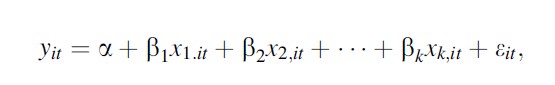Formula 1

where the dependent variable measures crime or recidivism and the independent variable measures the severity or the certainty of punishment.

This model has two possible interpretations:

1. Best linear predictor of Y
2. Conditional mean of Y given X

In order to get unbiased estimates of β=(β₁…β_k), one needs the measures of deterrence to be uncorrelated with the error term (in matrix notation E(x_kε)=0 for k=1…,K). According to the Gauss-Markov Theorem, if the rank condition is satisfied rank (x)=k and the variance of ε_i is σ² (homoscedasticity), then ordinary least squares (OLS) coefficients are the best linear unbiased estimators (BLUE). This means that the OLS estimator is the one with the highest precision (the lowest standard errors) among linear estimators.

Violations Of Ideal Conditions

The assumptions made by the Gauss-Markov Theorem can be violated by collinearity, omitted variable bias, simultaneity bias, measurement error, and heteroscedasticity.

Collinearity

When the explanatory variables are linearly dependent, for example, y=bx+az+e and x=wz, then y=(a+bw)z+e, so any linear combination of a and b is a solution to the OLS. It is always a good idea to look at the correlation matrix of all regressors. Whenever there is multicollinearity, a simple solution might be to reduce the number of explanatory variables, unless omitting variables causes biased parameter estimates.

Omitted Variable Bias

Suppose the true model is Y=Xβ+Zy+ε, but one estimates Y=Xβ+u, where u=Zy+ε. In this case β=E(X`X<sup>-1</sup>X`Y)+E(X`X<sup>-1</sup>X`Z)y+0. The bias is given by E(X`X<sup>-1</sup>X`Z)y. Notice that the bias disappears if the correlation between X and Z is zero (X`Z=0) or if the correlation between Y and Z is zero (y=0).

One example would be a recidivism (y) regression under alternative sanctions (x_i):

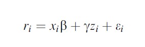Formula 2

where the omitted variable is unobserved criminal attitude (z). More criminally prone people might be more likely to recidivate and at the same time be less likely to receive alternative sanctions. How does one solve this issue? Notice that this bias is sometimes called selection bias and other times it is called endogeneity bias.

Measurement Error

One way to deal with omitted variables is to use proxies (variables that measure, even imprecisely, the excluded variable), in the previous example past criminal history, psychological reports, etc. However, proxies introduce a measurement error bias. If by adding decent proxies the coefficient β does not vary by much, one can be more confident about the OLS results.

Heteroscedasticity

The OLS estimator assumes that all the errors, eit , are identically distributed with the same variance for each unit of analysis (IID assumption). Based on this, it estimates the variance of the b coefficient. Since the condition rarely holds, the estimated standard errors of the estimated coefficients are different than the real ones. Since significance is based on the size of the standard error relative to the coefficient, this leads to an error in inference. Huber (1967) and White (1980)’s observation led to the Huber-White Sandwich estimator for the standard errors.

A similar issue arises when several units of observation can be grouped and their outcomes are correlated within the group. Taking into account this requires a clustering of the standard errors at the group level; see Moulton (1986).

Fixed Effect Estimation

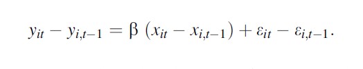
If the omitted variable is believed to be fixed across one dimension (time or space) and panel data (across time or space) are available, one can difference away the unobserved variable. Assume the model is

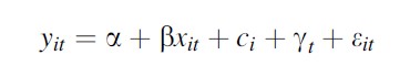Formula 3

With t and i fixed effects, the identification comes from changes within i and t. Forgetting about the t effects and averaging the model over t, one gets

Formula 4

With differencing one gets

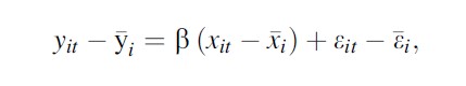Formula 5

which can be estimated by OLS. The alternative is to add individual fixed effects in the regression.

Another popular estimator that eliminates individual fixed effects is the first difference (FD) estimator:

Formula 6

One can show that the two estimators are the same when the total number of periods (T) is equal to two. When T≠2, whether one or the other estimators are preferred depends on the speed at which one thinks that x affects y.

Up until now one implicitly assumes fixed effects (intercepts) that might vary across individuals and marginal effect of X on Y (slopes) that were the same across individuals. But there are a variety of random effect/coefficient models that exploit distributional assumptions to estimate more complicated panel models, like

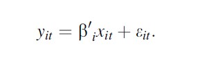Formula 7

The Counterfactual

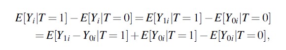
Before introducing individual-specific coefficients in more detail and to understand the potential endogeneity issue, it is often useful to think in terms of counterfactuals, especially when a policy is discrete or binary (0 or 1). Suppose one is interested in estimating whether more police reduces crime. Ideally one would increase the number of police officers, measure crime rates, and compare them to what would have happened had there not been an increase. The issue is that one does not observe this counterfactual. If Y_i measures crime rates in region i and T_i measures the treatment of an increase in police forces, one only observes Y_i =Y_i0(1-T_i)+Y_i1T_i meaning the crime rates in treated regions when treated and the crime rates in control regions when not treated.

Taking the simple average between treated and non-treated units

Formula 8

the first difference E[Y_1i -Y_0i |T=1] measures the average treatment effect on the treated (ATET), and the second difference E[Y_0i |T=1]- E[Y_0i |T=0] represents the selection, meaning the difference in outcomes between treated and non-treated regions in the absence of any treatment.

The identification of the treatment effect Y_i1-Y_i0 , the change in crime for the same region with and without more police, is all about finding a reasonable counterfactual, a control group, that eliminates the selection. Whenever there is random assignment of treatment, the treatment and the control group are statistically equivalent, and the simple difference in outcomes between the two groups E[Y|T=1]-E[Y|T=0]=E[Y₁-Y₀], is going to equal the average treatment effect (ATE). Randomized controlled experiments are rare in the economics of crime literature. Treatment is generally not randomly assigned due to cost or legal/moral objections, but rather assigned based on a policy or a change in policy. These policies often lead to discontinuities in treatment and can be seen as “quasi-experiments.”

But even if they were randomly assigned in such experiments, several problems can arise: (1) cost. These experiments tend to be very costly, which might reduce the size of the experimental group. (2) There might be noncompliance. Treated individuals/regions might decide not to get treated and the nontreated to get treated. (3) There might be nonrandom attrition among individuals when experimental units are observed over time. (4) The experiments might not last enough time to see a treatment effect. (5) The results of the experiment might not be generalizable (limited external validity). (6) There might be general equilibrium effects that would not be captured by an experiment.

Some of these limitations do not arise in “quasi-natural experiments.”

Quasi-Natural Experiments

Natural experiments are usually policy reforms or specific rules that can be exploited to measure exogenous changes in x. These interventions often change the treatment status of marginal participants, that is, those to whom treatment will be extended. Whenever treatment effects are not constant across participants, the treatment effects estimated on the marginal participants are called local average treatment effect (LATE) and may be very different from the treatment effects if the interventions had to be extended to the entire population. For example, incapacitation effects of incarceration are usually estimated based on the release of marginal prisoners (see Levitt (1996) and Barbarino and Mastrobuoni (forthcoming)). It would probably be incorrect to extend such estimates to the entire prison population, as marginal inmates should be less dangerous than inmates who keep on staying in prison. See Imbens and Angrist (1994) and Angrist et al. (1993), and see Heckman and Vytlacil (2005) for further discussion.

Depending on the “quasi-experiment” under study, there are different empirical methodologies that have been proposed to solve the endogeneity issues. The most commonly used are instrumental variables, regression discontinues, difference in differences, and reweighting techniques (propensity score and matching).

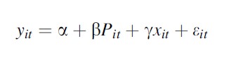
The Simple Difference

Suppose an outcome, for example, crime, y_it=a+βP_it +e_it depends on expected sanctions and that due to a policy reform, there is an across the board reduction in sanctions at time t, such that P_it =1 if t ≥τ and 0 otherwise. In this case, β=E(Y|P =1)- E(Y|P=0) measures the change in recidivism. If there are only two periods available, before (P =0) and after (P=1) the reform, the main assumption is that the only changes that happen over time are due to the reform. If more time periods are available, one can compare the evolution before and after the reform. One can also go beyond just analyzing the differences in means and look at quantiles. The main issue of such simple differences is that the changes might be due to other factors or that the reform was due to changes or expected changes in crime. In such case the reform variation would be endogenous.

The Matching And The Propensity Score Estimators

Whenever simple differences are the only available option, treatment and control groups need to be as similar as possible; otherwise simple differences might just stem from these differences and not depend on the treatment status. Whenever one thinks that these differences are driven by observable traits as opposed to unobservable characteristics, one can simply control for such factors (in this case we have selection on observables x):

Formula 9

An alternative is to compare individuals in the treatment group to individuals in the control group that have similar observable characteristics before treatment. Similarity can be defined based on the xs directly (e.g., nearest neighbor matching) or indirectly through likelihood of receiving treatment. The idea is that comparing individuals in the treatment and the control group that have the same estimated propensity to be treated should solve the selection issue. Once the likelihood of treatment (called propensity score) has been estimated, typically using logit or probit, there are several ways to match individuals in the two groups. Given the numerosity of matching procedures, it is important to show how robust the results are to the method used. In matching strategies, one pairs an individual in the treatment to one (one to one) or more (one to many) individuals in the control group, takes the difference in outcomes, and then averages across all treated individuals. For a discussion on efficiency, see Hirano et al. (2003). For an overview of matching estimators, see Smith and Todd (2001).

For such pairing to be even feasible, one needs a common support, that is, the range of propensities to be treated has to be the same for treated and control cases. This can be checked graphically by plotting the densities of the propensity scores by treatment status. If the overlap is not complete, one needs to limit the analysis to the smallest connected area of common support.

The propensity score can also be used to reweight observations in the control group such that their observable characteristics resemble on average the ones of the treatment group. Following Hirano et al. (2003), one can adjust for differences between the two groups by weighting observations by the (inverse) propensity score of assignment, that is, the probability of belonging to each group conditional on the observed covariates. Specifically, one can weight each unit by

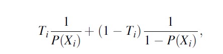Formula 10

where T_i is a dummy equal to 1 if the ith individual has been treated 0 otherwise and P(X_i) is the propensity score, meaning the probability of belonging to the treatment group conditional on the vector of individual characteristics X_i . The next section elaborates more on this approach.

The Synthetic Control Approach

Due to the increasing availability of micro data on victims and offenders, the matching and difference-in-differences estimators mentioned above often exploit variation over large samples of cross-sectional units observed over a few periods of time. In some cases, however, individual-level data are not available. Moreover, important phenomena such as organized crime, drug trafficking, and corruption involve significant spillovers between individuals within the same local area. Finally, most crime-prevention policies vary only at the aggregate level.

In all these cases, the available data usually include a few units (e.g., states or regions) observed over longer time periods. Synthetic control estimators provide a useful tool in this context because they match treated and control units on both the longitudinal and cross-sectional dimensions. The idea is to compare (difference in differences) each treated unit with a weighted average of control units that replicates the initial conditions in the treated unit many years before treatment.

This method was originally devised by Abadie and Gardeazabal (2003) to estimate the economic costs of terrorism in the Basque Country. They do so by comparing the GDP per capita of a region, Y_it with a weighted average of the GDP per capita in the other Spanish regions not affected by the

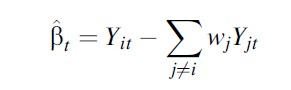Formula 11

where w_j is the weight attached to each jth region in the control group.

Following the notation of previous sections, Y_it=T_itY_1it+(1-T_it)Y_0it , where Y_1it and Y_0it is the potential GDP per capita with and without terrorism, respectively, and Tit is a treatment indicator for the presence of terrorism. After the outbreak of terrorism in the Basque Country, T_it=1 and T_jt =0 Ɐj ≠ i, so that

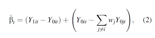Formula 13

where the first term on the right-hand side is the treatment effect of terrorism in region i and year t. The precision of βt depends thus on the difference between the synthetic control and the (unobserved) development of the treated region in the absence of the treatment (the second term on the right-hand side), so the estimation problem amounts to choosing the vector of weights that minimizes the last difference on the right-hand side of equation (2).

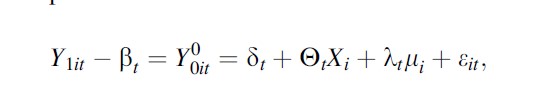
A natural choice consists in minimizing the same difference over the previous period, in which neither region had been treated (i.e., T_it =T_jt =0). As long as the weights reflect structural parameters that would not vary in the absence of treatment, the synthetic control provides a counterfactual scenario for the potential outcome Y_0it . Notice that an analogous identifying assumption, namely, that unobserved differences between treated and non-treated units are time invariant, is routinely imposed on difference-in-differences models. Indeed, Abadie et al. (2010) show that synthetic control methods generalize the latter by allowing the effect of unobserved confounders to vary over time according to a flexible factor representation of the potential outcome: conflict:

Formula 14

where δ_t is an unknown common factor with constant factor loadings across units, X_i is a (r×1) vector of observed covariates (not affected by the intervention), ʘ_t is a (1×r) vector of unknown parameters, λ_t is a (1×F) vector of unobserved common factors, mi is an (F×1) vector of unknown factor loadings, and the error terms ε_it are unobserved transitory shocks at the region level with zero mean. The traditional difference in differences imposes that λ_t is constant for all t’s.

Turning to the choice of the minimand, Abadie and Gardeazabal (2003) adopt a two-step procedure that minimizes the distance between the treated region and the synthetic control both in terms of pretreatment outcomes during the 1950s and a vector X of initial conditions over the same period (GDP per capita, human capital, population density, and sectoral shares of value added). Conditional on a diagonal matrix with nonnegative entries measuring the relative importance of each predictor, V, the optimal vector of weights W*(V) solves

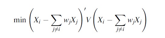Formula 15

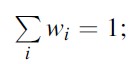
subject to w_i ≥0, Ɐi and

Formula 15A

 then, the optimal V * is chosen to minimize the mean squared error of pretreatment outcomes:

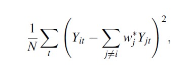Formula 16

where N_t is the number of years in the sample before the outbreak of terrorism.

After Abadie and Gardeazabal (2003), synthetic control methods have been used to study a wide range of social phenomena, including crime-related issues. As to the effects of (different types of) crime, Pinotti (2011) quantifies the costs of organized crime in southern Italy.

From a methodological point of view, Abadie et al. (2010) provide a throughout presentation of synthetic control estimators, while Donald and Lang (2007) and Conley and Taber (2011) propose alternative methods for dealing with small numbers of treated and control units in difference-in-differences models.

The Difference In Difference

If a new reform, or a new sanctioning rule, affects only some individuals (e.g., those in a given age group) but not others, a more convincing estimation strategy is to compare the changes in outcomes of the two groups. As in an experiment one can call the two groups the treatment and the control group. Estimating the following regression by OLS,

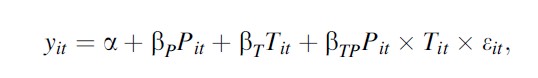Formula 17

where P defines the pre/post period and T the treatment group β_TP is called the difference-in-differences estimator. This estimator is equal to

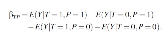Formula 18

The identification assumption is that the interaction between the reform and the treatment group is only due to the treatment or, in other words, that in the absence of treatment, the two groups would have shown similar changes in outcomes (parallel trend assumption). Generally this is more plausible when the two groups are similar in terms of observable characteristics and outcomes before treatment. One can usually improve these simple double differences performing robustness checks for the estimate, for example, using different control groups, looking at the evolution of outcomes over time, and exploiting sharp changes in treatment assignment.

One can also use difference-in-differences estimators coupled with matching estimators to reduce the initial differences between treatment and control groups (see, e.g., Mastrobuoni and Pinotti (2012)).

Instrumental Variables

Whenever one cannot credibly control for selection, researchers often start looking for an “exogenous variation” in x. Exogenous variations are usually driven by external factors (i.e., policy reforms, discontinuities in deterrence across individuals, across regions, or over time) that can plausibly thought to be unrelated to the dependent variable, other than through their influence on deterrence. Consider the model, where Z is an instrument for X: y=a+βX+ε.

For example, in the relationship between crime and police, a valid instrumental variable would be correlated with police but not with crime. Levitt (2002) used the number of firefighters as an instrument. If a one-unit change in the number of firefighters z is associated with 0.5 more police officers on the streets s and with a 100 decrease in total crimes, it follows that a oneunit increase in police officers is associated with -100/0.5 =-200 fewer crimes. Another instrument for police is the exogenous shift in policing resources that has been used in Draca et al. (2011).

The instrumental variable coefficient is

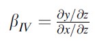Formula 18A

and can be estimated by two-stage least squares, regressing y on z and x on z and taking the ratio between the corresponding marginal effects

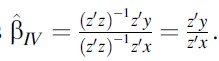Formula 18B

This simple formula can be generalized to the case of multiple regressors and multiple endogenous variables.

If one has more instruments than endogenous variables, one can test for overidentification. The intuition is that the estimated errors uˆ can be obtained excluding one instrument and then regressing it on the excluded instrument. Under the assumption H₀ that uˆ is consistent, one can test the exogeneity of the excluded instrument. In other words, such test rests on the assumption that for each endogenous variable, at least one instrument is valid.

It is important to always test for endogeneity of the explanatory variables. This can easily be done by regressing Y on X and on the corresponding predicted error term from the first stage, where one regresses X on Z. The t-statistic of the coefficient on the predicted error that is supposed to capture the endogeneity of X can be used to test endogeneity. The same test can be used for nonlinear second-stage estimation techniques such as probit or logit.

A final test that should be part of any IV estimation is related to the weak instruments issue. Instruments need to be correlated with the endogenous regressors, but whenever such correlation is too weak, it has been shown that the IV estimates converge to the OLS ones. The test statistics tend to be quite complicated, but in practice a simple rule of thumb is to have an F-statistic of the excluded instruments in the first stage (X on Z) that is larger than 10, though 15 seems to be a safer choice (see Stock and Yogo (2005)).

A special IV case is when z is a binary variable, (0; 1)

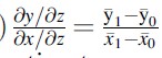Formula 18C

This estimator is called the Wald estimator.

Lochner and Moretti (2004) estimate the effect of education on crime by instrumenting education with compulsory schooling laws.

The Regression Discontinuity Design

Another difference estimator that is considerably more convincing than the simple one discussed above makes use of discontinuities in the assignment to treatment variable based on a, so-called, running or assignment variable. A classical example in the crime literature is the paper on deterrence and incapacitation effects by McCrary and Lee (2009). They use age of offenders as their running variable and age 18 as the threshold value where more punitive criminal sanctions take place (the treatment).

An important assumption is that individuals cannot manipulate the running variable and therefore assignment to treatment (they certainly cannot stop aging). In general one can examine the density of observations of the assignment variable around the threshold to test for manipulation McCrary (2008).

The other assumption is that at the discontinuity of the running variable, other variables, which might also be unobserved, do not change discontinuously. This means that unlike for the IV case, the running variable is allowed to influence Y but only in a smooth manner. There are two types of regression discontinuity (RD) design. In the first one, called the sharp design, as individuals move above the threshold, treatment status moves from 0 to 1 for everybody. In the second one, the conditional mean of treatment jumps at the threshold (fuzzy design).

The sharp design LATE estimate is equal to the average change in outcome at the discontinuity E(y⁺) – E(y^–), where “+” and “-” indicate observations just above and below the threshold. If in the fuzzy design the change in treatment is E(x⁺) – E(x^–), the local Wald estimator is [E(y⁺) – E(y^–)]/[ E(x⁺) – E(x^–]. Since the estimator is defined at the threshold, the main issue is about how to use the data efficiently without introducing too much bias, where the bias comes from moving away from the threshold. The default option is to run a regression of Y on local polynomials allowing for a jump at the threshold. The estimates are going to depend on the bandwidth choice (see McCrary (2008) for a discussion on this).

An RD design should start with a visual inspection of the discontinuity in treatment assignment. If such discontinuity is not clearly visible, a formal test that estimates [ E(x⁺) – E(x^–] should be reported. After the RD has been estimated, there are several tests that one can run to test the robustness of the results. One is to estimate the change in outcomes at random placebo cutoff points, and around 95 % should not be significant. One can also test whether other variables that should not be affected by the treatment show discontinuities at the threshold. One should also show how robust the results are to the choice of different bandwidths.

See Hahn et al. (2001) for an overview of the use of RD, and the special issue of the Journal of Econometrics (Imbens and Lemieux 2008a), and, especially, the practical guide by Imbens and Lemieux (2008b). Lee and Card (2008) explore the case when the regression discontinuity model is not correctly specified.

Bibliography:

1. Abadie A, Gardeazabal J (2003) The economic costs of conflict: a case study of the Basque country. Am Econ Rev 93(1):113–132
2. Abadie A, Diamond A, Hainmueller J (2010) Syntheticcontrol methods for comparative case studies: estimating the effect of California’s tobacco control program. J Am Stat Assoc 105(490):493–505
3. Angrist JD, Pischke J-S (2008) Mostly harmless econometrics: an empiricist’s companion. Princeton University Press, Princeton
4. Angrist JD, Imbens GW, Rubin DB (1993) Identification of causal effects using instrumental variables. NBER Technical Working Papers 0136, National Bureau of Economic Research, June 1993
5. Barbarino A, Mastrobuoni G (forthcoming) The incapacitation effect of incarceration: Evidence from several Italian collective pardons. American Economic Journal: Economic Policy
6. Cameron C, Trivedi PK (2005) Microeconometrics. Number 9780521848053 in Cambridge Books. Cambridge University Press, 3 2005
7. Conley TG, Taber CR (2011) Inference with difference in differences with a small number of policy changes. Rev Econ Stat 93(1):113–125
8. Donald SG, Lang K (2007) Inference with difference-indifferences and other panel data. Rev Econ Stat 89(2):221–233
9. Draca M, Machin S, Witt R (2011) Panic on the streets of London: police, crime, and the July 2005 terror attacks. Am Econ Rev 101(5):2157–2181
10. Hahn J, Todd P, Van der Klaauw W (2001) Identification and estimation of treatment effects with a regressiondiscontinuity design. Econometrica 69(1):201–209
11. Heckman JJ, Vytlacil E (2005) Structural equations, treatment effects, and econometric policy evaluation. Econometrica 73(3):669–738, 05 2005
12. Hirano K, Imbens GW, Ridder G (2003) Efficient estimation of average treatment effects using the estimated propensity score. Econometrica 71(4):1161–1189, 07 2003
13. Huber PJ (1967) The behavior of maximum likelihood estimates under nonstandard conditions. In: Proceedings of the fifth Berkeley symposium on mathematical statistics and probability, vol 1. University of California Press, Berkeley, pp 221–233
14. Imbens G, Lemieux T (eds) (2008a) The regression discontinuity design: theory and applications, vol 142. J Econom (Special issue). Elsevier, Feb 2008a
15. Imbens GW, Angrist JD (1994) Identification and estimation of local average treatment effects. Econometrica 62(2):467–475
16. Imbens GW, Lemieux T (2008b) Regression discontinuity designs: a guide to practice. J Econom 142(2):615–635
17. Lee DS, Card D (2008) Regression discontinuity inference with specification error. J Econom 142(2):655–674
18. Levitt SD (1996) The effect of prison population size on crime rates: evidence from prison overcrowding litigation. Q J Econ 111(2):319–351
19. Levitt SD (2002) Using electoral cycles in police hiring to estimate the effects of police on crime: Reply. Am Econ Rev 92(4):1244–1250
20. Lochner L, Moretti E (2004) The effect of education on crime: Evidence from prison inmates, arrests, and self-reports. Am Econ Rev 94(1):155–189
21. Mastrobuoni G, Pinotti P (2012) Legal status and the criminal activity of immigrants. Working Papers 052, “Carlo F. Dondena” Centre for Research on Social Dynamics (DONDENA), Universita` Commerciale Luigi Bocconi
22. McCrary J (2008) Manipulation of the running variable in the regression discontinuity design: a density test. J Econom 142(2):698–714
23. McCrary J, Lee DS (2009) The deterrence effect of prison: dynamic theory and evidence. Berkeley olin program in law & economics. Working paper series, Berkeley Olin Program in Law & Economics, July 2009
24. Moulton BR (1986) Random group effects and the precision of regression estimates. J Econom 32(3):385–397
25. Peracchi F (2001) Econometrics. John Wiley and Sons, Ltd., New York, NY
26. Pinotti P (2011) The economic costs of organized crime: evidence from southern Italy. Bank of Italy Working Papers
27. Smith JA, Todd PE (2001) Reconciling conflicting evidence on the performance of propensity-score matching methods. Am Econ Rev 91(2):112–118
28. Stock JH, Yogo M (2005) Testing for weak instruments in linear IV regression. In: Identification and Inference for Econometric Models: Essays in Honor of Thomas J. Rothenberg, eds Stock JH, Andrews DWK Cambridge University Press, New York, pp 109–120
29. White H (1980) A heteroskedasticity-consistent covariance matrix estimator and a direct test for heteroskedasticity. Econometrica 48:817–830
30. Wooldridge JM (2010) Econometric analysis of cross section and panel data, volume 1 of MIT Press Books. The MIT Press, June 2010

See also:

• How to Write a Research Paper
• Research Paper Topics
• Research Paper Examples

Free research papers are not written to satisfy your specific instructions. You can use our professional writing services to buy a custom research paper on any topic and get your high quality paper at affordable price.